Functors and Film Strips

stack_smileys

Summary

A video can be represented in two different ways: as a film strip, which lays out a sequence of frames across space, or as a movie, which lays out a sequence of frames across time. Each representation has its uses: editing a video as it’s playing is basically impossible; enjoying a video as a film strip is challenging. When needed, videos are (or used to be) edited by first turning them into strips of film, then editing the film, and then projecting the film as a movie. By implementing this process in Python and then describing it mathematically, we’ll reinvent the concept of functors, which are widely used in a branch of math called category theory and in functional programming languages like Haskell.

Film Editing 101

While working on a machine learning project recently, I ran into a common problem: the code base I wanted to work with made a few assumptions that didn’t fit my situation, and so it refused to run. Specifically, the code was written to work with image data, but I was working with movie data. That is, the code expected arrays with three dimensions, height, width, and color, but I was working with arrays with four dimensions, time, height, width, and color.

I resolved this problem by using the same trick as a video editor: I converted the movies into wide images, like strips of film, applied the code to them, and then converted the film strips back into videos.

To see how this works conretely, imagine we’d like to alter or edit video data that is available only as a movie.

First, let’s consider the movie-to-film process. If we have a movie and we want to convert it to film, we must record it, e.g. with a camera. Let’s abstract this process as capture, as in film = capture(movie).

At this point, we can apply any transformation that operates on films. For example, we can correct the colors, frame by frame, or we can add subtitles, which is much easier in less than real time. The result is an edited film, which we write edited_film = f(film), where f is a function that takes in film strips and returns film strips, here abstracting the human editing process.

Finally, we must convert the (edited) film strip back into a movie if we want to enjoy the fruits of our labor. This is done by projecting the film strip, by passing it in front of a synchronized light source that converts each frame in the strip into a projected frame in sequence. If we wanted to write this process the same way we did the previous two steps, we might write movie = project(film), where film can be any film strip whose aspect ratio matches the settings on our projection apparatus.

Film Editing for Pythons

Once we’ve agreed on a way to represent movies and film strips, we can go about writing a computer-friendly version of the editing process, which is both a nice springboard to thinking about it mathematically and a useful exercise to check our work. Computers are like diligent but not-too-bright students who listen to everything we say and nothing more, and bring nothing of their own to the table. If we cannot get them to understand it, we’re missing something in our description. This level of rigor is sometimes very useful.

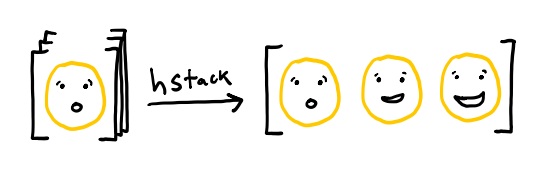
We begin with the capture process, which converts a movie into a film. There’s a convenient function in numpy that solves this for us: hstack, which takes an array of \(N\) dimensions and returns an array of \(N-1\) dimensions in which the first dimension has been “stacked” columnwise.

For example, matrices are two dimensional and vectors are one dimensional. So if we took the matrix np.eye(3), which is the identity matrix with three rows, and apply hstack, as below,

\[\begin{bmatrix} 1 & 0 & 0 \\ 0 & 1 & 0 \\ 0 & 0 & 1 \end{bmatrix} \xrightarrow{\texttt{hstack}} \begin{bmatrix} 1 & 0 & 0 & 0 & 1 & 0 & 0 & 0 & 1 \end{bmatrix}\]

we get as output the vector on the right. If we view the matrix as a sequence of rows, then the hstack transformation takes a sequence of short rows and returns a single very long row.

Similarly, we can provide a three-dimensional object, which is like a sequence of matrices, and get back out a very wide single matrix, as in the cartoon below.

stack_smileys

Note how similar the right hand side looks to a film strip! This means that the Python code is simple. Presuming we’ve imported numpy as np, we simply write

def capture(movie):
    film = np.hstack(movie)
    return film

Now to model “projecting” a film to get a movie. Reversing our description of hstack above, we need a function that converts a single, very wide array of dimension \(N\) into an array of dimension \(N+1\) that is like a sequence of less wide arrays of dimension \(N\).

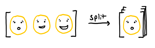
The numpy function that achieves this is called split. It needs to know which axis to split over and it needs to know the number of frames, but then it does exactly what we want, as shown in the cartoon below

split_smileys

Because we chose to use hstack, which stacks across columns, we know that axis=1, the column axis in numpy. The other argument, the number of frames, is a bit trickier.

It can’t be inferred just from the film strip, at least as we’ve done it. Though real film strips have regions separating each frame, ours do not. Therefore, the projectionist, looking at our smiley video as a strip of film, has no way of telling whether it’s meant to be a simple movie of a smiley going from surprised to happy or a more avant-garde movie showing two halves of a face flickering from side to side.

smiley_dilemma

By making assumptions on what kinds of videos are likely to come through, we could try to infer the location of the splits, but that would require us to make judgment calls, which might make our system break for, e.g., the hand-painted films of Stan Brakhage. Since we don’t want to disenfranchise anybody, we instead restrict our projector to operating with a fixed aspect ratio. From the aspect ratio and the height and width of the film strip, we can deduce the number of frames. If we later have videos with different aspect ratios, we can just define more projectors.

The resulting Python code is a bit more involved than our capure code:

def project(film):
    aspect_ratio = 1  # projector settings
    frame_height, film_width, _ = film.shape
    num_frames = film_width / height / aspect_ratio
    movie = np.split(film, num_frames, axis=1)
    return np.asarray(movie)

But the majority of our effort is just spent on computing the number of frames. One small gotcha: split returns a list of equal-sized arrays, which is subtly different from an array that has those arrays as sub-components. To avoid this, we need to use asarray to convert the list into an array.

Now that we can convert films to movies and vice versa, it’s time for the magic step, which lets us convert any function that operates on films (with a fixed aspect ratio) to a function that operates on movies:

def convert_to_movie_function(film_function):
    def movie_function(movie):
    	edited_movie = project(film_function(capture(movie)))
    	return edited_movie
    return movie_function

This is the way to express, in Python, the very intuitive idea that we can watch an edited movie by converting the movie to film (capture), editing the film (film_function), and then projecting the edited film as a movie (project).

You should stop a moment to think about how you might write convert_to_film_function, which takes a movie_function and returns a film_function.

Generalized Abstract Nonsense

Now that we’ve worked through a concrete example, both intuitively and more rigorously, through programming it, we’re ready to think abstractly about this problem.

Our “editing” process was really just almost any transformation of the film that didn’t change its aspect ratio (for the diligent, restrict to pure, computable, total functions that preserve aspect ratio).

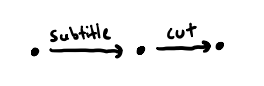
Imagine drawing each valid film as a dot on a piece of paper, and then drawing an arrow pointing from a film to its edited version. Mathmetically, a collection of dots and arrows between them is called a graph. A small example appears below, showing a film, its subtitled version, and the version that has been subtitled and cut down to a shorter running time, connected by the relevant arrows.

film_cat

Briefly thinking in Python terms again, notice that if subtitle and cut are functions whose inputs and outputs are valid films, then we can always define a function subtitle_then_cut, that looks like

def subtitle_then_cut(film):
    return cut(subtitle(film))

whose inputs and outputs are always valid films, and so our previous drawing was missing an arrow.

film_cat_compose

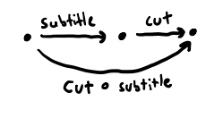
Combining two functions into one by applying one after the other is called composition. If the functions are \(f\) and \(g\), applied in that order, we usually write \(g \circ f\) for their composition, which we might pronounce “\(g\) after \(f\)”. Alternatively, we might write \(f . g\), pronounced “\(f\) then \(g\)”.

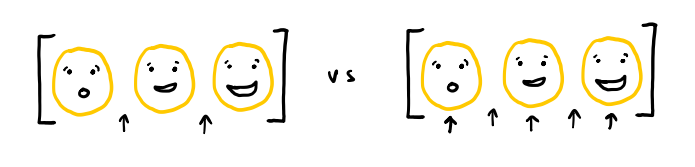
Now imagine drawing the collection of all valid movies in a similar way. Rather than starting over again, build it from the film diagram. Start with the dots. They correspond to the projected versions of each film. How do we determine the arrows?

We can generate an arrow in our movie diagram by using convert_to_movie_function to take an arrow between films and create an arrow between movies. A diagram of this process appears below:

film_functor

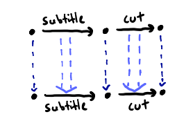
Dashed arrows represent parts of this process; single blue arrows represent the action of capture; double blue arrows represent the action of convert_to_movie_function.

Notice that we haven’t included the arrow for cut \(\circ\) subtitle. By our argument above, that arrow can be inferred from the arrows in the simpler diagram, so drawing it is superfluous. This is one of the reasons mathematics is interested in rules, which we might frame more positively as guarantees. They allow us to be more succinct without losing clarity, at least in principle.

Another thing to notice is that that missing arrow is missing from both diagrams; that is, we also have a cut \(\circ\) subtitle arrow for movies. Returning to our concrete implementation, consider the difference between convert_to_movie_function(subtitle_then_cut) and the function convert_to_movie_function(cut) \(\circ\) convert_to_movie_function(subtitle). The latter will repeatedly convert back and forth between film and movie, while the former will only do that twice: once at the beginning and once at the end of the editing pipeline.

If we can confirm a rule, or provide a guarantee, that the two functions are identical, then we can write a faster, perhaps much faster, version without losing anything. If we were software engineers designing an editing interface, we’d know that we can take arbitrary-length lists of editing steps and turn them into a single function with only two conversion steps (ponder: how did we go from two functions to an arbitrary number? hint: composition).

If we become more precise in stating our assumptions, we can say that the collection of all valid films and the editing procedures that convert one into another form a category, a structure from abstract mathematics that encompasses just about all cases where some kind of composition “makes sense”. A mapping that takes one category, e.g. films and edits, and associates it to another category, e.g. movies and edits, is called a functor, just like a mapping between two sets is called a func tion. The only restriction is that the functor must preserve composition, meaning that in our film example convert_to_movie_function(subtitle_then_cut) and convert_to_movie_function(cut) \(\circ\) convert_to_movie_function(subtitle) are the same function, just implemented differently. Writing the names of the functions as \(f\) and \(g\), and writing our functor as \(\Phi\), pronounced “fee”, we can write this condition as

\[\begin{align} \Phi(f) \circ \Phi(g) = \Phi(f \circ g) \end{align}\]

Functors abound in the world of computer science. There is a functor between data and lists of data, which Python folks may have come across as a list comprehension: a function that takes in the elements of the list and returns elements is used to create an expression that acts on the list and returns a list.

Summary

Film Editing 101

Film Editing for Pythons

Generalized Abstract Nonsense

More Relevant Reading