How Long is a Matrix?
\(\begin{align} \lvert\lvert X\rvert\rvert^2_2 = \mathrm{tr}\left(X^\intercal X\right) \end{align}\)
Summary
This blog post sets out to provide an answer to two questions: how long is matrix? what is the distance between two matrices? Doing something somewhat silly, unraveling the matrix into a vector and computing the length of that vector, turns out to be a good choice; furthermore, it turns out to be connected to the notion of singular values, and provides an explanation, of sorts, for the ubiquity of terms like \(X^\intercal X\) and \(\mathrm{tr}\left(X^\intercal Y\right)\) in certain areas.
Spaces of Vectors Have Nice Properties
Spaces of real-valued vectors come equipped with an intuitive notion of length: add up the square of each component, then take the square root. This also leads to an inutitive notion of distance between vectors, the length of the difference between them. This is the Euclidean distance. This notion of distance has the major benefit of being invariant to rotations and reflections, which means that distances and lengths don’t change when you turn your head upside-down or look in a mirror.
By a leap of insight, we can also define the similarity between two vectors by recognizing the square as a product of two identical numbers and “relaxing” it to a product of different numbers. Dropping the square root, we get the inner product, which can be normalized to give the cosine similarity.
Can We Extend Those Properties to Spaces of Matrices?
A space of matrices (all of the same size) is itself a “vector space” in the abstract sense: it satisfies the axioms of closure, addition, scalar multiplication, &cetera. Note that there is an unfortunate overloading of terms here, since a vector can either mean 1) a one-dimensional array of numbers or 2) an element of a vector space, which could be a single number, an \(N\)-dimensional array, or even a function.
One would hope that the space of matrices has all the same nice properties as the space of vectors: it comes with a notion of distance, that notion of distance is invariant to changes of basis, and so on.
We Can, and It’s Not Even That Hard
Indeed, we can make a perfect correspondence (each matrix is mapped to one vector and every vector has an associated matrix; this is an isomorphism) between matrices of size \(M\) by \(N\) and vectors of length \(M\cdot N\): simply “ravel” or “vectorize” the matrix by writing its elements out in a one-dimensional array.
This suggests a devious, if somewhat facially silly, method for determining the length of a matrix: map it to its associated vector, then measure the length of the vector. This method is called a “pullback”, since we are using our correspondence to “pull” the notion of length back from the space of vectors and into the space of matrices.
This seems too inelegant to possibly work. But it does, and the result has the hifalutin’ name Frobenius norm.
The Resulting Quantity Admits a Simple Representation
To prove anything, we need to start writing formulas.
We denote the length, or norm, of a matrix or vector \(X\) with straight brackets \(\lvert\lvert X\rvert\rvert\). Thus our definition of the norm is
\(\begin{align} \lvert\lvert X \rvert\rvert &\colon = \lvert\lvert \mathrm{vec}\left(X\right) \rvert\rvert\\ &= \sqrt{\sum_{ij} X_{ij}^2} = \sqrt{\sum_{ij} X_{ij}\cdot X_{ij}} \end{align}\)
Carrying around all those square roots is tedious and currently unimportant, so let’s work with the squared norm, which we write \(\lvert\lvert X\rvert\rvert^2\).
Our goal is to express this quantity in a manner that is independent of the basis in which we write the matrices, so this coordinate-centric (i.e. index-laden) representation isn’t going to cut it.
Let’s try to express our formula as a native operation on matrices. We only have a few tools at our disposal, namely scalar multiplication, and matrix addition and multiplication, and transposition, so we begin with those.
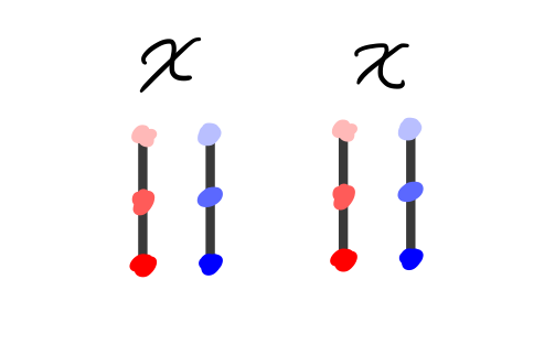
The first pass would be to multiply \(X\) with itself. This is, unfortunately, a non-starter, since our matrices need not be square, and so it need not be the case that they can be multiplied. See the diagram below, for a running example with 3-by-2 matrices.
But an element of a vector space and its transpose can always be multiplied (the dimensions of the multiplication become \(N\) by \(M\) and \(M\) by \(N\)), so we instead try multiplying \(X^\intercal X\).
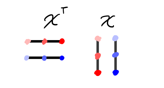
The result now has the sum of the products of the elements of each column \(i\) in \(X\) with each other column \(j\) in \(X\) in its position \(ij\) (see diagram below). Note that this matrix is square and symmetric.
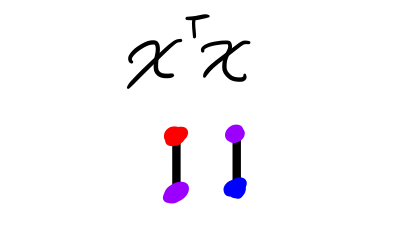
But we only wanted to multiply like elements with each other – \(X_{12}\) with \(X_{12}\), and so on – so we need to extract only the diagonal elements of \(X^\intercal X\) and then add them up.
This operation is also called the trace, represented with \(\mathrm{tr}\).
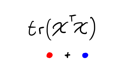
Therefore we can write our squared norm as
Note that this is emphatically not a computational prescription for computing the squared norm. \(X^\intercal X\) includes a number of terms that are irrelevant for that calculation (in general, many more irrelevant than relevant terms). We are writing things this way in order to learn something about the quantity we are computing, not to compute it.
From That Representation, We Can Prove Nice Properties
Now we need to start flexing our linear algebra muscles. We’d like to show that we can apply a rotation or reflection, also known as an orthogonal transformation, without affecting the value of the norm.
A matrix \(R\) is orthogonal if \(R^\intercal R = RR^\intercal = I\), where \(I\) is the identity matrix.
If we apply an orthogonal transformation to \(X^\intercal X\), we see that the squared norm becomes
Unfortunately, our \(R\) and \(R^\intercal\), which we know we can cancel, are separated by other terms. If only we could change the order of the expression inside the trace, then we would have the desired result.
And in fact, the trace is invariant to reorderings: \(\mathrm{tr}\left(AB\right) = \mathrm{tr}\left(BA\right)\). To save space, I refer you to this math Stack Exchange post for the (short) proof.
So we choose \(B=R\) and get
just as we’d hoped.
And Show a Connection to Eigenvalues
Things get even better! Notice that we’ve shown that the trace is invariant to orthogonal transformations: our proof made no use of the properties of \(X^\intercal X\), other than that it was square.
Note further that every square, symmetric matrix is diagonalizable: there exists an orthogonal transform such that the matrix can be written as a diagonal matrix, \(\Lambda\), with the eigenvalues \(\lambda_i\) along the diagonal.
Because the trace is invariant to orthogonal transformations, then, we know that the trace of the original matrix is equal to the trace of its diagonal form, and so
And so, from our embarrassingly obvious definition of the length of a matrix in terms of the length of its vectorized form, we’ve arrived at a more subtle, but equivalent definition: the squared length of a matrix \(X\) is equal to the sum of the eigenvalues of \(X^\intercal X\). Because this matrix is symmetric and real, its eigenvalues are real. In fact, \(X^\intercal X\) is positive semi-definite (proof here), meaning that its eigenvalues are all non-negative. This proves that our notion of length cannot be negative, which is nice.
These eigenvalues appear sufficiently often that they are studied in their own right. Their square roots are the the singular values of the matrix \(X\), traditionally represented by the symbol \(\sigma\). They are so similar to eigenvalues that they were originally called eigenvalues (and, in fact, eigen is German for “singular” or “specific”), but luckily the name didn’t stick.
From this notion of length, we can get a notion of distance between matrices by subtracting and then computing length, just as we did for vectors.
We Can Relax this Notion of Length to Get an Inner Product
Recall that the inner product of vectors \(x\) and \(y\) was defined by “relaxing” the expression \(x^\intercal x\) into \(x^\intercal y\). What happens if we perform the same substitution as above?
If you look carefully over the arguments above, you’ll notice that we only start using properties of \(X^\intercal X\) that are not shared by \(X^\intercal Y\) fairly late in the game. The former is symmetric, and so diagonalizable, while the latter is not, and so is not necessarily diagonalizable.
Forunately enough, there exists a “relaxation” of diagonalizability that only requires that the matrix by square: the Jordan Canonical Form. In this form, which is also related to the original matrix by an orthogonal transform, the eigenvalues still appear on the main diagonal, but they are now (possibly) joined by \(1\)s on the first upper diagonal.
But the argument about the trace being the sum of the eigenvalues still holds. Of course, the matrix \(X^\intercal Y\) is not necessarly positive semi-definite, so the inner product is no longer non-negative, but inner products are allowed to be negative, and so no need for tears.
Normalized versions of this inner product result in a notion of cosine similarity of matrices.
Singular Values Also Show Up in Other Notions of Matrix Size
There are other norms on spaces of vectors: the sum of the absolute values, for example, or the largest entry in the vector. Many of these norms are so-called \(\ell_p\)-norms, since they correspond to choosing powers \(p\) other than \(2\). These norms are critical for analyzing such spaces. Can we also extend these to spaces of matrices?
The shortest answer is yes. A slightly longer answer is as follows: the equivalents of these norms for matrices are called Schatten \(p\)-norms, and the norm we’ve discussed so far is, in fact, the Schatten 2-norm.
But are these norms still connected to singular values? The full answer is enough material for a separate post, but the beginnings of the connection can be concisely stated.
The most interesting matrix norms arise as answers to the question “what does applying this matrix to a vector do to its norm?”. That is, we ask about the quantity
questions like “what is the largest value this quantity can take? the smallest?” and so on. But that quantity, known as the Rayleigh quotient, can be rewritten
The answer to all our questions about the Rayleigh quotient, then, can be answered by looking at the eigenvalues of \(X^\intercal X\), bka the singular values of \(X\), though now we are interested in their largest and smallest values, their sum, and so on.
And We Learned a Lesson Along the Way
Have we learned any mathematical lessons in this process, besides the brute facts? I think this approach demonstrates the power of the pullback/pushforward method: even when your isomorphism is kind of silly and certainly not all that mathematically respectable, it can still give reasonable answers. My all-time favorite instance of this method is probably “How the Simplex is a Vector Space”, which beautifully ties together log-probabilities and probabilities in an unexpected way. I also quite enjoyed using pushforwards to succinctly state the business of statistics.
These kinds of abstract, algebraic/categorical approaches can be a breath of fresh, clean air, even (or perhaps especially) in situations where the details seem overwhelming and salient.