Linear Algebra for Neuroscientists

The Importance of Linear Algebra

Linear algebra is one of the most important workhorses of applied mathematics. Linear algebra is critical in statistics, optimization, geometry, and more. It shows up whenever we need to consider a collection of numbers as a single object, and just one of many such collections, all of the same length. This turns out to be super common: for example, the x, y, and z coordinates of an object in three-dimensional space are such a collection, as are the firing rates of a population of neurons.

Linear algebra is just as important for neuroscience as it is for any other scientific field that uses math. Even though neurons and neural circuits have complex, non-linear behavior, we need the tools of linear algebra to describe that behavior.

Unfortunately, despite its critical importance, linear algebra just isn’t sexy, so it is often taught perfunctorily and by someone who’d rather be teaching something else to students who’d rather be learning something else. The result is that a lot of folks dislike linear algebra and find it more of a confusing stumbling block than a useful tool.

These notes present a few core concepts of linear algebra – vectors, matrices, and dot products – in a manner that neuroscientists will find intuitive, in an effort to clear away some of that confusion.

My hope is that this will encourage folks to dive deeper into other resources for learning linear algebra, whether in a neuroscience context, like in Kenneth Miller’s short textbook or in a more general context, as in Khan Academy’s online course. Readers interested in an intuitive presentation of the core ideas of linear algebra should check out Grant Sanderson’s YouTube Lectue Series, which pairs lucid explanations with slick animations and graphics.

A Simple Neural Circuit

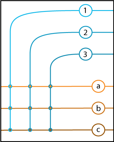
As our neural circuit model, let’s take the parallel fiber and Purkinje cell circuit of the cerebellum. In order to get a clean, cartoon picture, we focus on a collection of three parallel fibers (below, in shades of blue, labeled 1, 2, and 3) that are all connected to each of three Purkinje cells (below, in shades of orange, labeled a, b, and c).

The dendritic inputs for the parallel fibers enter from the right, while the inputs of the Purkinje cells enter from left. The axons of the parallel fibers turn and pass over the dendrites of the Purkinje cells, synapsing with each of them in turn (indicated by colored circles).

We will assume that these neurons form a linear system. What this means is that if the input to a neuron is doubled, or multiplied by any number, the output of the neuron doubles, or is multiplied by that same number. Also, if we measure the outputs of a neuron for two inputs separately, then we know the output of the neuron for those two inputs together: it is the sum of the outputs to the separate inputs.

The first property is called scaling and the second property is called superposition. Real neurons don’t have either of these properties – as a very rough example, multiplying the input current to a neuron by seven million won’t cause the output to be seven million times greater, it’ll just fry the neuron – but our cartoon neurons do. This will make it possible for us to write down precisely how our neurons behave.

Experiment #1: Measuring the Behavior of a Single Neuron

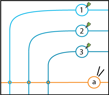
Let’s perform some thought experiments on our cartoon neurons. First, let’s place our imaginary recording electrode (indicated by two almost-intersecting lines, representing our pipette tip) on Neuron \(a\) and shine our imaginary laser (indicated by the green lightning bolts) on Neurons 1, 2, and 3, which we’ve modified using optogenetics so that they respond to light by increasing and decreasing their activity. The experiment is depicted below.

If we stimulate Neuron 1 to fire some unit amount, we will measure some rate of firing from Neuron \(a\). That is, when Neuron 1 is firing at a rate of 1, we measure some firing rate from Neuron \(a\). Loosely speaking, we can think of that value as a synaptic weight for the synapse between Neuron 1 and Neuron \(a\). Our assumption that scaling inputs causes outputs to scale by the same amount (the scaling assumption) lets us take that synaptic weight and use it to predict the output rate of Neuron \(a\) in response to any input rate in Neuron 1.

Indicating the output of Neuron \(a\) as \(\text{out}_a\), the firing rate of Neuron 1 as \(\text{in}_1\), and the synaptic weight between Neuron 1 and Neuron \(a\) as \(a_1\), we can write a simple equation for the output of Neuron \(a\) as a function of the input from Neuron 1:

\(\text{out}_a = a_1 \cdot in_1\)

Plugging in a few numbers will verify that this equation is correct: when Neuron 1 is not firing, Neuron \(a\) won’t fire, and when Neuron 1 is firing at a rate of 1, the firing rate of Neuron \(a\) is \(a_1\), just as we measured it before.

Notice the similarity of this equation to the equation for a line of slope \(m\) and intercept of 0:

\[y = mx\]

this is why our neurons are linear neurons: if we graph their outputs as a function of their input, we get a line!

We can repeat these measurements for Neurons 2 and 3, and we will get three equations that will let us predict the output of Neuron \(a\) in response to separate stimulation of each input neuron.

\(\text{out}_a = a_1 \cdot \text{in}_1 \\ \text{out}_a = a_2 \cdot \text{in}_2 \\ \text{out}_a = a_3 \cdot \text{in}_3 \\\)

With these three equations, we can now predict the output of Neuron \(a\) in response to any input! We just need to use our other assumption, the superpositioning assumption. That assumption told us that the response of a neuron to the combination of two inputs is just the sum of the outputs to the two inputs individually. Written out mathematically, in our case, that means:

\(\text{out}_a = a_1 \cdot \text{in}_1 + a_2 \cdot \text{in}_2 + a_3 \cdot \text{in}_3\)

We can shorten this equation substantially by writing

\[\text{out}_a = \sum_i a_i \cdot \text{in}_i\]

where \(i\) goes from \(1\) to \(3\).

While these ways of writing the behavior of our linear neuron work, they have their flaws: the first is too long, while the second is too short. We’d like a notation that reminds us of which numbers are multiplied with which, but without all the extra \(+\)’s and \(\cdot\)’s.

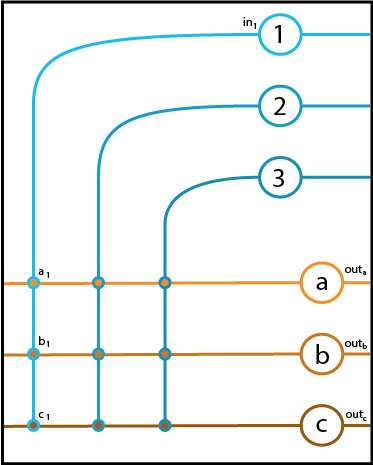
If we write the seven relevant numbers down on our picture of the circuit (as seen below), a neat spatial layout for the equation suggests itself:

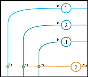
\(\left[\begin{array}{c} a_1 & a_2 & a_3 \end{array}\right] \left[\begin{array}{ccc} \text{in}_1 \\ \text{in}_2 \\ \text{in}_3 \end{array}\right] = \text{out}_a\)

To compute the output, we take a pair of elements in turn, one from each of the boxes, and multiply them together. Once that is done, we add the three results up to get our output. The result of each multiplication is the component of the firing rate of Neuron \(a\) that is due to the activity of a single neuron, and the superposition principle lets us add them all up.

The two boxes are called vectors. For obvious reasons, the one on the left is a row vector and the one on the right is a column vector. We might call them \(\vec{a}\) and \(\vec{\text{in}}\), where the arrow is intended to remind us that, even though we’re using only one symbol, we’re referring to a collection of multiple numbers. The process of multiplying two vectors together is variously known as

• the dot product, because it can be written \(\vec{a}\cdot\vec{\text{in}}\) (notice the dot)
• the scalar product, since the result is a single number, also known as a “scalar” because multiplying by a number “scales” things
• a weighted sum, since we multiply each element of \(\vec{\text{in}}\) by a value, or weight, from \(\vec{a}\). Note that this has nothing directly to do with “synaptic weights”; we could also think of the output as a weighted sum of the values from \(\vec{a}\) with weights given by \(\vec{\text{in}}\).

These operations are ubiquitous in mathematics. For example, computing the average of a collection of \(N\) numbers is a multiplication of vectors: one vector containing all of the numbers and the other containing \(1/N\) in each position (this operation is a good example of a weighted sum). In the greatest generality, even derivatives and integrals are a form of vector multiplication.

Rather than diving deeper into those ideas, we’ll return to our neural circuit to see how recording the outputs of more than one neuron at a time leads us to matrices.

Experiment #2: Measuring the Behavior of Multiple Neurons

In many neuroscience contexts, the behavior of a single neuron is not very informative. Instead, it is the behavior of many neurons together that gives rise to the behavior of the system. This view gave rise to the philosophy of connectionism and thereby the artificial neural networks that have been so successful in solving problems with computers that previously only humans and animals had been able to solve.

So let us proceed to measuring the responses of all three of our output neurons, \(a\), \(b\), and \(c\), simultaneously, and see what happens.

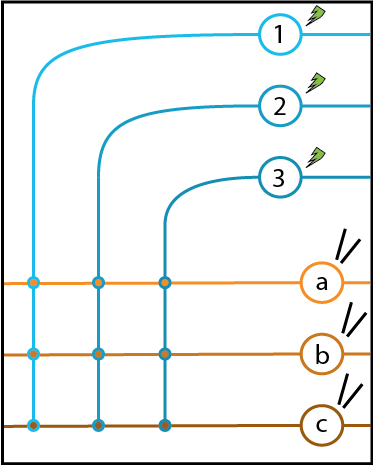
A cartoon of this experiment appears below, with green lightning bolts indicating optopgenetic stimulation and black lines indicating the positions of recording electrodes.

Since our output neurons (in orange) are not connected to each other, we can repeat the same stimulation experiment we used on Neuron \(a\) above to get the synaptic weights from Neuron 1 to each of our output neurons.

That is, we stimulate Neuron 1 to fire at a unit rate and record the output rates of the three neurons. These three rates become the values of our synaptic weights \(a_1\), \(b_1\), and \(c_1\). A diagram of this stage of the experiment appears below.

As before, we can now predict the responses of our three output neurons to any input rate from Neuron 1. The three equations appear below.

\(\text{out}_a = a_1 \cdot \text{in}_1 \\ \text{out}_b = b_1 \cdot \text{in}_1 \\ \text{out}_c = c_1 \cdot \text{in}_1 \\\)

As before, we can summarize these equations with a vector equation, which is valid so long as Neuron 1 is the only active input:

\(\text{in}_1 \cdot \left[\begin{array}{ccc} a_1 \\ b_1 \\ c_1 \end{array}\right] = \left[\begin{array}{ccc} \text{out}_a \\ \text{out}_b \\ \text{out}_c \end{array}\right]\)

This equation tells us that firing in Neuron 1 is “broadcast” into firing in Neurons \(a\) - \(c\) with different weights (but remember, nothing prevents one or more of the weights from being \(0\)).

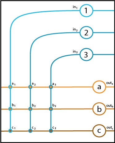
To complete our study of this neural circuit, we repeat this for input Neurons 2 and 3. The result is that we have recovered all of the synaptic weights and can predict the output of our circuit in reponse to arbitrary input patterns.

First, a diagram of the circuit, with the synaptic weights added:

If we compare this to the diagram we had at the end of our first experiment, the interpretation that jumps out at us is that we have three equations, one for computing the output of each neuron. These equations are:

Once again, the repeated structure of these three equations suggest that we can combine them into a more compact notation, just as we did with the equations that described how to calculate the output of Neuron \(a\).

For starters, we can use the “dot product” notation to emphasize that the weights and inputs are vectors – collections of indexed numbers. This gives us:

\(\text{out}_a = \vec{a} \cdot \vec{\text{in}} \\ \text{out}_b = \vec{b} \cdot \vec{\text{in}} \\ \text{out}_c = \vec{c} \cdot \vec{\text{in}} \\\)

But notice the inefficiencies and inadequacies of this representation: the input vector, \(\vec{\text{in}}\), is repeated three times, and the output, which is a vector, is split into three separate equations.

If we look again at the diagram of the circuit above, an alternative, spatial notation, much like the one that initially inspired us to introduce vectors, suggests itself: we take the three synaptic weight vectors of neurons \(a\) - \(c\) and combine them into a 2-dimensional object by stacking them on top of each other. Then, we calculate the output of each neuron by taking the corresponding row of this 2-d array and multiplying each of its elements by the corresponding input firing rate.

We can write this as:

\(\left[\begin{array}{ccc} a_1 & a_2 & a_3 \\ b_1 & b_2 & b_3 \\ c_1 & c_2 & c_3 \\ \end{array}\right] \left[\begin{array}{ccc} \text{in}_1 \\ \text{in}_2 \\ \text{in}_3 \end{array}\right] = \left[\begin{array}{ccc} \text{out}_a \\ \text{out}_b \\ \text{out}_c \end{array}\right]\)

The 2-d array of numbers is called a matrix. Make sure to look between this equation and the circuit diagram and see what patterns jump out at you! Notice how much more natural and sensible the rules for multiplication are in this context, compared how they are normally taught.

Just as we summarized our one-dimensional arrays, our vectors, with a single symbol by placing an arrow over the top of a letter, we can summarize our matrix with a single symbol. The standard is to use a single, Latin capital letter that is not italicized. Sometimes, boldface letters are used. Choosing the symbol \(\textbf{W}\) for our matrix of synaptic \(\textbf{W}\)eights, we end up with

\[\vec{\text{out}} = \textbf{W}\vec{\text{in}}\]

as our final equation describing the behavior of this circuit. In this form, the similarity to the equation for a line with zero intercept, \(y = mx\), is emphasized, as is the fact that the entire behavior of the circuit depends on just the synaptic weights.

The preceding discussion focused on our first vector equation, which summarized how to calculate the output of a single linear neuron with multiple inputs. The operative vector was a row vector, the vector of weights of neuron a, and this led us to a view of the weight matrix that was row-centric.

We can instead return to our second vector equation, the one from the perspective of Neuron 1, reproduced below:

\(\text{in}_1 \cdot \left[\begin{array}{ccc} a_1 \\ b_1 \\ c_1 \end{array}\right] = \left[\begin{array}{ccc} \text{out}_a \\ \text{out}_b \\ \text{out}_c \end{array}\right]\)

in this equation, the operative vector is a column vector (corresponding to a column of our matrix). Instead of describing what the output of a single neuron looks like in response to multiple inputs, this equation describes what happens to input from a single neuron as it produce multiple outputs.

This gives us a second perspective on our matrix: while the rows correspond to the transformations that output neurons perform on input vectors, the columns correspond to the result of stimulating a single input neuron.

This perspective interacts nicely with our two principles for linear systems: superposition and scaling. Any combination of firing rates in the input neurons can be described as a superposition and scaling of single input neurons firing at rate \(1\). That is, we can think of an input vector \(\left[ 2,\ 4,\ 0 \right]\), as the superposition of the first input neuron firing alone at rate \(1\), scaled by \(2\), and the second input neuron firing alone at rate \(1\), scaled by \(4\), and the third input neuron firing alone at rate \(1\), scaled by \(0\).

Vectors with one element equal to \(1\) and all the others equal to \(0\) are called canonical basis vectors: basis vectors because superpositions and scalings of those vectors can be equal to any vector of the same length and canonical because they are the simplest, most obvious vectors that are a basis.

Therefore our second perspective on the weight matrix \(\textbf{W}\) is that its columns correspond to the output in response to the canonical basis vectors. Try working through the matrix-vector multiplication yourself for a particular canonical basis vector and this fact should pop out at you.

Conclusions

\(\left[\begin{array}{ccc} a_1 & a_2 & a_3 \\ b_1 & b_2 & b_3 \\ c_1 & c_2 & c_3 \\ \end{array}\right] \left[\begin{array}{ccc} \text{in}_1 \\ \text{in}_2 \\ \text{in}_3 \end{array}\right] = \left[\begin{array}{ccc} \text{out}_a \\ \text{out}_b \\ \text{out}_c \end{array}\right]\)

This blog post aimed to explicate the somewhat unintuitive matrix equation above, with its seemingly arbitrary rules for who gets multiplied with whom and what gets added where, in terms of a system that neuroscientists might find intuitive: a simple neural circuit. This encouraged us to take two views of this matrix equation, one from the view of our output neurons, which emphasized the rows of our matrix, and one from the view of our input neurons, which emphasized the columns of our matrix.

These ideas just begin to scratch the surface of linear algebra. What began, as it did here, as a simple notational convenience, has blossomed into an indispensible tool of both applied and pure mathematics. I hope that, armed with the intuition from this neural circuit example, neuroscientists feel more comfortable chasing those more abstract and complex features of linear algebra. Grant Sanderson’s Essence of Linear Algebra video lecture series is a great way to start!