Answer
This post assumes a solid background in the biophysics of the membrane potential, in particular the "equivalent circuit" for the neuron, and the leaky integrate-and-fire neuron model. Go back and read those if you get lost below!
Extending Our Neuron Models
In previous posts on, e.g., the ionic basis of membrane potentials I've made a few simplifying assumptions about neurons.
One of the most common and least explicit involved the shape of neurons. In order to make our derivation of the Nernst equation possible, we assumed that the neuron was a sphere – even more, we assumed that we could treat it as flat from the perspective of an ion (just as we assume the Earth is flat from the perspective of a dropped ball when we do physics problems).
Neurons, like the Earth, are not flat (pace B.o.B.). They are also not even approximately spherical. They extend through space in a complicated fashion.

Fig. 1 A cartoon neuron, the Earth, and a flat sheet. None of these are actually spherical, though some are better approximated by spheres than others. Photo of the Earth from nasa.gov.
The complexity of these shapes makes it much harder to make confident, general statements, as we have before, about the flow of currents and the effects of forces. The simplicity of our model also makes it impossible to say anything about things like currents passing through dendrites.
But we need not throw our hands up in despair! We just need to replace our rough, spherical model with a more sophisticated model!
We'd like our model to still be easy to work with: in particular, we'd like our equivalent circuits to fit nicely into it. Luckily, there's just such a model available: we can use cylinders instead of spheres! (Why are the electronics of cylinders well-described and easy to work with? Think wires!)
The figure below shows our cartoon neuron on the left, and then our new, better approximation, constructed from cylinders and spheres, on the right.
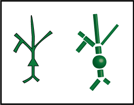
We call each cylinder or sphere a "compartment". Each compartment has its tiny copy of the equivalent circuit, and directly connected compartments have connected circuits. Current can flow between these compartments, with the strength depending on how they are connected.
A Refresher on the Leaky Integrator Equation
We can see how currents flow in our new-and-improved neuron models by reusing the leaky integrator equations that we used to describe our simplest computational neuron model.
The basic leaky integrator equation appears below. I've modified it a bit from its form in the original post.
This is a differential equation. That means that it describes how a variable changes over time. The symbol for "changes over time" is \(\frac{d}{dt}\), where d stands for "tiny change". The variable that changes is V.
The right side of the equation describes just how V changes with time.
Each g stands for a conductance, which is the inverse of a resistance. Our conductances are our ion channels; the more that are open, the higher the value of g.
Each E stands for an equilibrium potential, or the potential at which a current driven by some electrochemical potential will have no net flow.
With these terms defined, we're now ready to determine what happens to V. The first term involves our "leak" conductances and their equilbrium potential. Since these "leak" conductances are open at rest, their equilibrium potential is called the "resting membrane potential". The first term says that whenever V is less than \(E_{leak}\), V goes up, and it goes faster the larger \(g_{leak}\) is – the more leak channels we have open. If V is higher than \(E_{leak}\), V goes down. In both cases, the first term is 0 whenever V is equal to \(E_{leak}\). So this term just captures what we mean by "resting membrane potential": it's the potential at which the neuron "rests", or doesn't change its voltage.
The second term looks a bit more intimidating, but it's just as simple as the first. Now, instead of concerning ourselves with the "leak" conductances, we're concerned with other ionic conductances, like the AMPA current for excitatory inputs or the chloride current for inhibitory inputs. For each of these conductances, we look at how far V is from the equilibrium potential, E, of the conductance, and then we weight that by how many channels are open, g. We do this for all of our different kinds of channels, and then add the result up.
There's one last piece: on the left-hand side, we have a number \(\tau\). \(\tau\) controls how quickly V changes. If \(\tau\) is big, then V changes slowly. \(\tau\) is determined by the over-all conductance and capacitance of the neuron.
Putting It Together: Leaky Compartment Models
Let's extend our leaky integrator equation from above to handle our new-and-improved compartmentalized neuron model. The below figure shows a cartoon model, the compartment approximation, and then a representation of the compartment model as a graph.
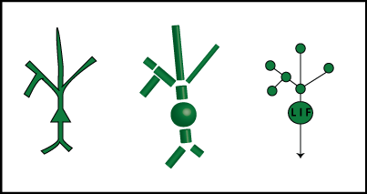
The nodes of the graphs are the compartments, and the edges represent connections. We call a set of directly connected nodes a "neighborhood". For now, each node from the dendrites is just a leaky integrator, while the soma has the ability to fire action potentials – it's an "LIF" or "leaky integrate-and-fire" node.
With this representation in hand, we can add a term to our leaky integrator equation to represent the influence of neighboring compartments:
Our additional term is very similar to our original two: whenever the compartment we care about has a voltage different from its neighbors, the compartment's voltage will move towards the neighbors. We weight the connection to each neighbor n with a value \(c_n\), which tells us how well-connected two compartments are. If the compartments aren't very wide where they connect, \(c_n\) will be small. Note also that the time constant, \(\tau\), will be different for each compartment. The value of \(\tau\) is determined by the shape, size, and electrical properties of the compartment.
How Do Electrical Signals Propagate or Dissipate Through the Dendritic Tree?
The equation above answers this question in detail for any given dendritic tree: currents change the voltages of neighboring pieces of the neuron, dissipating more when the branches are thin and long, or when certain pieces are poorly connected to each other, as in dendritic spines.
Before we declare victory, let's note that: there's no action potential generation in our model. Because LIF neurons have no natural spike-generating mechanism, we can't capture back-propagating action potentials or dendritic spikes, which are important phenomena for learning and memory, and can generally substantially increase the computational power of a single neuron.
Our compartmental model would still be central to any approach for incorporating thse phenomena, but our neuron model would have to become more complicated.