Hypothesis Testing
| $$2+2=5$$ | $$2+2\neq5$$ | |
|---|---|---|
| Tails | $$0$$ | $$0.5$$ |
| Heads | $$0$$ | $$0.5$$ |
To celebrate the latest stable version of Applied Statistics for Neuroscience, here’s a tutorial on hypothesis testing, based on the lecture notes for the course. Make sure to check out the whole course if you liked this snippet!
Hypothesis Testing
This tutorial covers the basis of hypothesis testing, including null hypotheses, error types, error rates, and \(p\)-values. These will require us to develop some fundamental ideas from probability, including joint, marginal, and conditional probabilities.
If you’d like a more thorough-going introduction to these ideas, along with an introduction to Bayes’ Rule for relating them to each other, check out this blogpost.
Hypothesis Testing is a Kind of Decision-Making Under Uncertainty
Inferential statistics is concerned with a particular kind of inference problem: trying to infer the value of a parameter, like the average value or spread of some random variable in a population. Examples of random variables and populations include:
- neural firing rate and mouse somatosensory neurons
- whether an individual smokes or not and Canadians under the age of 25
- the mean of the data you measured in your experiment and the collection of all datasets you could’ve measured
The purpose of such inferences is to guide decision making. For example, we might measure the average response of a sick population to a candidate drug and then use that value to determine whether to prescribe the drug or not. We left unsaid, however, just exactly how statistical inferences are to be used.
In this tutorial, we’ll work through how to use statistical inferences to guide the simplest kinds of decisions: yes-or-no decisions, also known as binary decisions, since there are two choices. We’ll focus on the yes-or-no decision of most interest to scientists: is my hypothesis true or not?
Binary Hypothesis Testing
In an experimental science context, a binary hypothesis is an answer to a question that usually looks something like: “does this intervention have an effect?” Examples include:
- Do neurons subjected to trauma express different levels of protein XYZ?
- Does adding distractors increase reaction time in healthy human subjects?
- Does optogenetically stimulating neural circuit A change the activity of neural circuit B?
Each of these questions has a yes or no answer: “yes, the intervention has an effect” or “no, the intervention has no effect”. We call these answers hypotheses. The hypothesis that the intervention has no effect is called the null hypothesis, while the hypothesis that the intervention has an effect is called the alternative hypothesis. These are frequently written as \(H_0\) and \(H_A\), with \(0\) and \(A\) standing for for “null” and “alternative”.
When we answer a binary question, there are two possible answers: yes and no, which we call the “positive” and “negative” answer. Furthermore, either the alternative or the null hypothesis could be true. Therefore, there are four possibilities, which appear in the table below:
| Truth is $$H_A$$ | Truth is $$H_0$$ | |
| We claim $$H_A$$ | True Positive | False Positive |
| We claim $$H_0$$ | False Negative | True Negative |
The nomenclature for each of these four events is intuitive: the first word is “true” or “false” depending on whether out answer was correct or incorrect (not, e.g., whether the alternative hypothesis is true or false) and the second word is “positive” or “negative” depending on what we claimed.
The historical names for the off-diagonal elements of this chart, which correspond to incorrect assertions or “errors”, are “Type I Error” and “Type II Error”. These names are not to be preferred, since they literally correspond to the (arbitrary) order in which the kinds of errors were described in an early paper by Neyman and Pearson. As such, they have no descriptive power, unlike “false positive” and “false negative”.
However, they are frequently used, so consider the following mnemonic, which is floating about the internet, unattributed: “when the boy cried wolf, the villagers committed a Type I and a Type II error, in that order”.
Example: Touching Cat Feet
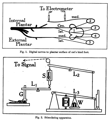
Let’s work through a quick example from one of the early Nobel Prizes granted to a neuroscientist, ED Adrian. Take our alternative hypothesis to be “pressing a weight onto a cat’s hind foot causes increased firing in the nerve exiting the foot”. The alternative hypothesis, then, is that no such increase in firing occurs. The figures depicting the experimental apparatus from Adrian and Yngve’s 1926 paper testing this hypothesis appear below.
The simplest test we might perform to determine the veracity of this hypothesis is to first measure the firing rate of the sensory nerve when the foot is not being stimulated, then measure it again when the foot is being stimulated. We take the difference of these two values, and we accept the alternative hypothesis if the value is less than \(0\).
Let us assume, as we often do with hypotheses that have won Nobel prizes, that this hypothesis is true. If we measure a higher rate in the foot after it is pressed and therefore claim that the alternative hypothesis is true, we have a true positive result. If, despite the veracity of the alternative hypothesis, we measure a lower firing rate in the stimulated foot (due to uncontrolled fluctuations in the firing rate, like those due to ion concentration changes, changes in ambient temperature, movement by the experimental subject, etc.), and therefore claim that the null hypothesis is true, then we have a false negative result. If the alternative hypothesis that stimulation of the foot with a weight increases firing rate were instead false, and we measured no difference in firing rate, or a difference in the opposite direction, then we would have a true negative result. Lastly, we could measure an increase even if the hypothesis were false, again due to uncontrolled factors, and the result would be a false positive.
Note that if we had designed our test differently, we might expect the chances of different outcomes to change. For example, we are certainly free to design a really bad test, like measuring things the exact same way we did above, but claiming the opposite of what our experimental findings suggested. Note that this wouldn’t always work to our deteriment: all of our false positives would become true negatives, for example. More sensibly, we might take ten measurements of each condition, then compute the averages before subtracting. Or we might phrase the null hypothesis differently, like “the increase in firing rate is less than 10%”. We see intuitively that this is better design, but we don’t know how much better. If we want to better understand the outcomes of our hypothesis tests, we need to be more rigorous about how we design our experiments, state our hypotheses, and make our decisions.
Making Hypothesis Testing Rigorous
At a high level, in statistical hypothesis testing, we take some data and use that to determine whether we claim \(H_A\) or \(H_0\). The key insight that lets us think rigorously about statistical hypothesis testing is to treat both the correct answer (columns in the above table) and the answer we give (rows in the above table) as uncertain quantities, as random variables.
It may seem strange to think of our claims about the world as being random, since random is used colloquially to mean “arbitrary” or “without structure or meaning”. But recall that anything we calculate from randomly-sampled data “inherits” some randomness from that data – its value can be different each time we collect a dataset. Because our decisions are based on our data, they can be different from experiment to experiment. Put another way, the result of calculating something based on data is a statistic, and statistics have sampling distributions, as discussed in the earlier material.
The “correct answer” also isn’t random in the sense that most people think of randomness. However, it’s also not random in the sense described above: a statement like “this intervention has an effect” is either true or false, and it doesn’t change whether it’s true or false depending on the data we collect. Instead, we recognize that we aren’t entirely certain whether “this intervention has an effect” is true or not, and we instead write down a number that captures the degree to which we believe that the statement is true: a logically true statement like \(2+2=4\) is associated with the number \(1\), while a logically false statement like “This number is greater than itself” is associated with the number \(0\). All other kinds of statements, like “It will rain tomorrow” or “Extraterrestrial life exists” fall somewhere in between. We call this number the probability that the statement is true.
The view that randomness arises from sampling is a core component of the frequentist view of statistics. The view of that randomness arises from uncertainty is a core component of the Bayesian view of statistics. We’ll avoid being dogmatic in this course, switching freely between the views whenever one or the other is simpler.
Joint Probabilities
Now that we have two different random variables, the outcome of our testing procedure and the ground truth, we can think of the probability that any pair of events occurs, where the first element of a pair comes from the first random variable and the second element comes from the second random variable.
If we shorten the events to \(+\) and \(-\) for the outcome and \(T\) and \(F\) for the correct answer (where \(T\) means the alternative hypothesis is true), we write a table just like the one above to store the probabilities of pairs of events:
| $$T$$ | $$F$$ | |
|---|---|---|
| $$+$$ | $$p(+,T)$$ | $$p(+,F)$$ |
| $$-$$ | $$p(-,T)$$ | $$p(-,F)$$ |
where \(p(+,T)\) should be read as “the probability the test is positive and the alternative hypothesis is true”. Since these probabilities tell us the chance that two events both occur, we call them joint probabilities. The table above is called a joint probability table. The information it stores is called a joint probability distribution. In this case, the distribution is a mass function, since it tells us the probabilities of discrete events.
A joint probability distribution is a powerful thing. As we shall see below, we can use it to determine how to interpret the outputs of our statistical tests: does a negative result imply a high probability that the hypothesis is false? if the hypothesis is true, what is the chance that the test comes up negative? These are crucial questions that fundamentally change how we interpret and use our tests.
Let’s leave aside the question of where the joint distribution comes from. For now, let’s say we know all of these numbers, and see what they imply. We’ll use a running example with the joint probability table below. Notice that these numbers add up to 1 – that’s what makes the values a valid probability distribution.
| $$T$$ | $$F$$ | |
|---|---|---|
| $$+$$ | $$0.5$$ | $$0.15$$ |
| $$-$$ | $$0.05$$ | $$0.3$$ |
Marginal Probabilities
First, we can use the joint probability table to figure out the probabilities of the individual random variables that make up the table. For example, we can figure out the probability that the alternative hypothesis is true.
We do this by simply adding up the probabilities of all events in which the alternative hypothesis is true. In this case, there are two such events: the alternative hypothesis is true and we claim it is true \((+,T)\) and the alternative hypothesis is true and we claim it is false \((-,T)\). These events correspond to the cells in the first column. Similarly, we can calculate the probability that the alternative hypothesis is false by adding up the values in the second column or calculate the probability of each outcome of our test by adding up the appropriate row.
Below, you’ll find these values are worked for our example table. There, as traditionally, the probability of an event is written at the end of the column or row corresponding to that event. These areas are called the margins and so these probabilities are called marginal probabilities. Notice that if we add up the marginal probabilities along a row or column (the numbers with a particular background color), the result is 1. That means these are probability distributions – the marginal probability distributions of the test outcome and the alternative hypothesis.
| $$T$$ | $$F$$ | $$p(\text{test})$$ | |
|---|---|---|---|
| $$+$$ | $$0.5$$ | $$0.15$$ | $$0.65$$ |
| $$-$$ | $$0.05$$ | $$0.3$$ | $$0.35$$ |
| $$p(H_A)$$ | $$0.55$$ | $$0.45$$ |
There’s nothing magical happening here. We could’ve made the rows correspond to a different random variable, like whether it’s raining in Kansas or whether Mercury is in retrograde. After all, the total chance that the alternative hypothesis is true is equal to the chance that it is equal and Mercury is in retrograde plus the chance that it is equal and Mercury is not in retrograde (it might be helpful to think in terms of frequencies here). Calculating marginal probabilities from a joint probability table is just an accounting trick to make more obvious the information that’s already in the table.
The marginal probability distribution of the alternative hypothesis is of particular importance. It tells us what we believe about the world before we take into account the result of our statistical test. For this reason, it’s called the prior probability of the hypothesis. There is some degree of subjectivity in setting prior probabilities, since they arise from complex, fuzzy factors related to our fundamental beliefs about the world (are our educated guesses usually right or usually wrong? is nature usually simple or usually messy?) and the combined results in the literature.
Conditional Probabilities
The joint probability table told us the chance that any particular pair of events occurs, while the marginal probability distributions told us the chance that any individual event occurs, irrespective of the other variable in the pair.
Often, however, we know the value of one of the variables. For example, once we’ve run the statistical test, we know what the outcome turned out to be. Other times, we would like to assume that one of the variables takes on a particular value (e.g. that the null hypothesis is true) and determine how the probability of each outcome for the other variable has changed. Do we need to throw out our old, possibly hard-won, joint probability table and start over?
Luckily, the answer is no. Using the joint probability table, we can construct two new tables, which tell us the probability distribution of one of the random variables for fixed values of the other. Because the probabilities in these tables only pertain when a certain condition is satisfied (these probabilities are conditional on the other random variable having a certain value), they are called conditional probability tables.
How do we determine the values in these tables? Consider the right column of the joint probability table above, corresponding to all cases where the alternative hypothesis is false. This column almost tells us the conditional probabilities. For example, we can readily see that when the alternative hypothesis is false, the probability that the test comes up negative is twice the probability that it comes up positive (\(0.3\ =\ 2\cdot0.15\)).
However, \(0.3 + 0.15\) doesn’t equal \(1\) – it’s equal to \(0.45\), so we can’t just directly use those numbers for the conditional probabilities. However, if we divide them by their sum, they’ll add up to \(1\):
\[\frac{0.3}{0.3+0.15} + \frac{0.15}{0.3+0.15} = \frac{0.3+0.15}{0.3+0.15} = 1\]Put another way, the rows and columns of the joint probability table are like un-normalized conditional distributions – distributions that don’t add up to one. To make them into proper distributions, we need to normalize them by dividing by their sums, which happen to correspond to the marginal probabilities.
The two conditional probability tables for our running example appear below. One corresponds to viewing the rows of the joint table as un-normalized distributions (and so conditioning on test outcome, the random variable in the rows of the table) while the other corresponds to viewing the columns as un-normalized distributions (and so conditioning on the truth value of the alternative hypothesis, the random variable in the columns of the table).
| $$T$$ | $$F$$ | ||
|---|---|---|---|
| $$+$$ | 0.77 | 0.23 | $$p(H_A\lvert +)$$ |
| $$-$$ | 0.14 | 0.86 | $$p(H_A\lvert -)$$ |
| $$T$$ | $$F$$ | |
|---|---|---|
| $$+$$ | 0.91 | 0.33 |
| $$-$$ | 0.09 | 0.67 |
| $$p(\text{test}\lvert T)$$ | $$p(\text{test}\lvert F)$$ |
The vertical bar, \(\vert\), is pronounced “conditioned on” or “given”. One would read the expression \(p(\text{test}\vert T)\) as “the conditional probability distribution of the test outcome given that the alternative hypothesis is true”.
Note one important difference between a conditional probability table and a joint probability table: while the latter is a distribution, the former is NOT. For example, the entries of a conditional probability table don’t add up to 1. Instead, each row or column of a conditional probability table adds up to 1. A conditional probability table is a collection of distributions, with one distribution for each value of the variable being conditioned on.
Because of this distinction, there are several entities that end up getting called “the conditional probability”. For example, the first table above is “the conditional probability of the alernative hypothesis given the test outcome”, \(p(H_A\lvert \text{test})\). The first row in that table is “the conditional probability of the alternative hypothesis given that the test is positive”, \(p(H_A\lvert \text{test}=+)\). The first cell in that row is “the conditional probability that the alternative hypothesis is true given that the test is positive”, \(p(H_A=T\lvert\text{test}=+)\).
Unfortunately, depending on the context, the mathematical shorthand for all three of the above can be \(p(x\vert y)\), with the meaning depending on which of \(x\), \(y\), or both are outcomes (e.g. “test is positive”) and which are random variables (e.g. “the outcome of the test”). Sometimes this ambiguity is resolved by denoting random variables with capital letters and their outcomes with lowercase letters, but this can be overly restrictive.
Conditional Probabilities and Hypothesis Testing
We introduced joint probabilities in order to understand hypothesis testing. Now that we are armed with the two conditional probability tables associated with the joint probability table, we can start to dive deeper. Let’s start with the row-wise conditional probability distributions.
The “Test-Interpretation” Table
| $$T$$ | $$F$$ | |
|---|---|---|
| $$+$$ | $$p(T\lvert +)$$ | $$p(F\lvert +)$$ |
| $$-$$ | $$p(T\lvert -)$$ | $$p(F\lvert -)$$ |
Because these probabilities are conditioned on the outcome of a test, they tell us how to interpret the results of a test that we have performed.
Consider the top row of this table. This row tells us the conditional probability of the alternative hypothesis when we’ve gotten a positive test result. Notice that \(p(T\vert +)\) isn’t \(1\) – a positive test result doesn’t mean that we are now 100% certain that that the alternative hypothesis is true. In the case of our running example, it’s \(0.77\).
Recall that we already had a number that reflected our belief that the alternative hypothesis is true: the prior probability of the alternative hypothesis. The conditional probability table above tells us how we should update that belief when we see the result of the test. Since these probabilities come after we collect data and perform a test, they are called posterior probabilities.
Posterior and conditional probabilities are very general concepts. Because of the importance of binary hypothesis testing, the conditional probabilities in the table above have special names that capture their role in interpreting tests. Those names are:
| $$T$$ | $$F$$ | |
|---|---|---|
| $$+$$ | Positive Predictive Value | False Discovery Rate |
| $$-$$ | False Omission Rate | Negative Predictive Value |
where coloring, as above, indicates conditioning on the same value. Because of this, two named quantities with the same background color must add up to 1, and so knowing one tells you the other. Depending on the context of the problem, one will be easier or harder to think about.
The positive predictive value was described above. The term false discovery rate arises from considering what would happen if we ran a particular test many times. The false discovery rate tells us the fraction of our positives that would be false positives (or false discoveries, when the alternative hypothesis being true means the discovery of a new phenomenon or drug).
The values in the second row mirror the values in the first row. The negative predictive value tells us the posterior probability that a negative test result reflects the truth – higher values mean that negative results on the test are more meaningful. The false omission rate is akin to the false discovery rate, but it tells us the fraction of our negatives that are false negatives, or incorrect omissions of certain phenomena or candidate drugs from our list of real or effective ones.
Next, let’s consider the column-wise conditional probability distributions.
The “Test-Design” Table
| $$T$$ | $$F$$ | |
|---|---|---|
| $$+$$ | $$p(+\lvert T)$$ | $$p(+\lvert F)$$ |
| $$-$$ | $$p(-\lvert T)$$ | $$p(-\lvert F)$$ |
Because these probabilities are conditioned on whether the alternative hypothesis is true or false, they don’t tell us how to interpret the results of a test. Instead, they tell us how the test will perform in situations where the hypothesis is true and where it is false. Notice that the diagonal values correspond to the probability that the test gives you the right answer in each case. These probabilities are useful for folks who design statistical tests: without having to worry about whether the alternative hypothesis is likely to be true or false, they can confirm that their test is useful by ensuring that the diagonal elements of the above table are both large.
As above, these quantities have special names to distinguish them from run-of-the-mill conditional probabilities. Because they are more commonly used and used by a wide array of disciplines, they have multiple names, the most common of which appear below.
| $$T$$ | $$F$$ | |
|---|---|---|
| $$+$$ | True Positive Rate, Power, Sensitivity | False Positive Rate, α |
| $$-$$ | False Negative Rate, β | True Negative Rate, Specificity |
Take care when interpreting the terms that end in rate, like “true positive rate” and “false negative rate”. The temptation is to interpret them as referring to the fraction of your tests that are true positives/false negatives. This is incorrect. Instead, these rates tell you the fractions of such tests in situations where the alternative hypothesis is true. That is, if we know the alternative hypothesis is true, then we can use the true positive rate to tell us how many of our tests should be true positives. The false positive rate and true negative rate tell us the false positive and true negative fractions in situations where the null hypothesis is true.
At first, these numbers seem to be of limited use for scientists, since we certainly wouldn’t be doing experiments if we knew whether the hypothesis was true or false!
The utility of this table is that it doesn’t require us to specify \(p(H_A)\), so we can avoid all of the difficulties described above for figuring out prior probabilities. The rightmost column of this table is particularly easy to calculate, so it has long dominated the design of hypothesis tests. To make things a bit more concrete, we now turn to how we calculate the values in this column and use them to design a test.
Good: Hypothesis Test Design Using \(p(+\lvert F)\)
Example: Adrian and Yngve
Let us return to our neuroscience example: we wish to test the hypothesis that pressing on a cat’s hind foot causes an increase in the firing rate of the nerve exiting the foot.
Imagine that we knew the probability distribution of firing rates that we measure in the case where the foot is not being stimulated. For example, we might have collected thousands of trials, so we have a very good estimate of this probability distribution. Given a new measurement value, we might like to know how likely it was that we’d get that value. Unfortunately, the answer to that question for a continuous value like firing rate is always \(0\), as discussed in the earlier section on probability density functions. Instead, we have to ask how likely it was that we’d measure a firing rate around that value, or at least as large or small as that value. In both cases, we take an area under the curve given by the probability density function.
A key insight that lets us rigorously design a statistical test here is that if the null hypothesis is true, then the distribution we measured for the firing rates in the nerve of the unstimulated foot is exactly the distribution of the firing rates in the stimulated foot, under the null hypothesis. This distribution is often called the null distribution. Armed with this distribution, we can calculate the chance that we would observe a firing rate at least that large if the null hypothesis were true. It’s simply the procedure described above: take the probability distribution given by the observations of the unstimulated foot and measure the area under the curve that is at or above the measured value.
The resulting number is the chance, under the null hypothesis, that we would collect the data that we collected. This is a famous number. It is called the \(p\)-value. The lower this value is, the less likely it is that we would observe the data that we observed under the null hypothesis. Put another way, if this value is low and the null hypothesis is true, then our results are very surprising – they represent some sort of cosmic coincidence. Science, and much of rational inference, rests on the assumption that being less surprised is better and bizarre coincidences don’t occur that often. All else being equal, if another hypothesis results in us being less surprised by the information we have, then we prefer that hypothesis.
We can use the \(p\)-value to design a statistical test whose false positive rate we know exactly. If we reject the null hypothesis and claim that the alternative hypothesis is true whenever the \(p\)-value is less than some number α, then our false positive rate will be α. It’s helpful to spell out exactly why. Remember that the \(p\)-value is the chance that we would observe the data we observed under the null hypothesis. By definition, half of time, we’ll measure \(p\)-values that are under \(0.5\) – in this case, we can be explicit and say that half of the data we observe should be at least as large as the median. This same argument holds for each percentile.
Summary
Let’s abstract a bit from the example given above.
The general principle that we used to determine whether a test was a good choice or not was that if an event occurs that is too unlikely to occur under a given hypothesis, then we discard that hypothesis. The event we focus on is the value of a statistic, a function of our data, which we call the test statistic. Good test statistics usually have two properties:
- We know their sampling distribution under the null hypothesis
- That distribution has a single peak, with values falling off quickly on either side
The second property lets us say that the event we’re interested in determining the likelihood of is observing an extreme value of the test statistic, where extreme usually means far away, in either direction, from the peak of the sampling distribution, but could mean far away in a particular direction. The first property lets us figure out what the likelihood of that extreme event is. This likelihood is called the \(p\)-value (or, more accurately, \(p\)-statistic). Once we’ve done that, we compare our \(p\)-value to some pre-selected value α (the common, but my no means compulsory or necessary, choice is \(0.05\)), and if the observed value is lower, we reject the null hypothesis.
If we’re not interested in determining the \(p\)-value exactly, but just want to know the outcome of our test, we can use the sampling distribution of the test statistic under the null hypothesis (also known as the null distribution of the test statistic, for “short”) to calculate the value of the test statistic that will be extreme enough to be just under our pre-selected value. We call this value the critical value of the test statistic.
The only difference between the simple test we described above and even very complex statistical tests is that our choice of statistic was very simple: the value of a single observation. For most modern experiments, this test is not good enough – for example, the chance of a true positive might be almost 0! Let’s improve our design process for statistical tests by looking at some of the other entries in our conditional probability tables.
Better: Hypothesis Test Design Using \(p(-\lvert T)\)
Because both columns of our “test-design” conditional probability table must add up to \(1\), there are really only two independent entities. Above, we covered one of those, the false positive rate and its twin, the true negative rate.
The other pair is the false negative rate and its twin, the true positive rate. The true positive rate is also known as the power, so this section might also be titled “Power Analysis”. For reference, we reproduce the conditional probability table here:
| $$T$$ | $$F$$ | |
|---|---|---|
| $$+$$ | True Positive Rate, Power, Sensitivity | False Positive Rate, α |
| $$-$$ | False Negative Rate, β | True Negative Rate, Specificity |
The critical difference between this column (on the left) and the column considered above (on the right in the table) is that, where previously the event being conditioned on was that the null hypothesis was true, now, the event being conditioned on is that the alternative hypothesis is true.
Just as before, if we want to calculate the numbers in this column, we need to know the distribution of our test statistic under the hypothesis we’re assuming is true. Unfortunately, this is much more complicated in the case of alternative hypotheses than for null hypotheses. One cause of this is that the null hypothesis is very specific: “there is no effect of this intervention on the measured variable”. Another way to phrase this, using more technical language, might be “the size of the effect of this intervention is \(0\)”. The alternative hypothesis is often less specific.
Consider our running example: the null hypothesis was that there was no change in the firing rate between nerves coming from stimulated and unstimulated cats’ feet. That is, the change in firing rate caused by stimulating the foot with a weight was \(0\). The alternative hypothesis was not so specific: we hypothesized that there was a change, but we didn’t say how big it was. That is, we didn’t specify an effect size.
This makes it difficult to figure out how likely we are to make a false negative error. If the effect of stimulation on firing rate is tremendously large, then the chance of a false negative is lower – it’d take a very large coincidence of uncontrolled factors to “cancel it out” and make us erroneously conclude that the null hypothesis was true. If the firing rate change is extremely small, then a false negative is extremely likely – we need the uncontrolled factors to coincidentally break in the same direction as the intervention in order to reject the null.
This underscores the importance, however, of calculating a true positive rate. Science experiments are expensive and time-consuming, and it would be wasteful to perform experiments for which there is little hope of getting the correct result. For a sobering account of the issues caused by the widespread failure to account for the true positive rate, check out Button, Ioannidis, et al., 2013.
In order to calculate the true positive rate, we need to specify the distribution under the alternative hypothesis, which usually means specifying an exact value for the size of the effect that we believe we’ll find. This raises two issues. First, we need to determine how we specify that value. Second, we need to calculate the true positive or false negative rate from that value.
The solution to the first problem is straightforward, if rarely done outside of certain contexts like large clinical trials or very expensive, long-running experiments. We run a very small experiment, also known as a pilot, and calculate an effect size from that experiment. We don’t care whether the effect was significant or not; we simply use it as an estimate of the true effect size. This gives us a specific alternative hypothesis to test and so gives us, in principle, a sampling distribution of the test statistic under the alternative hypothesis.
The second problem is a bit tougher. Though pre-written methods for calculating the distribution of many test statistics under various null hypotheses are widely available, methods for calculating these distributions under alternative hypotheses are harder to come by. Firstly, there is less demand, since the scientific community has historically been less aware of the importance of calculating true positive rates. Awareness has spread, but roll-out of this kind of power analysis software is limited. For example, the availability of such packages for Python is quite limited. Secondly, calculating the sampling distribution for a specific value of the effect is often quite involved, often more so than for the absence of an effect. The difficulty is increased if, as is often desirable, we want to say “the effect is no bigger than \(a\) and no less than \(b\)”.
Best: Hypothesis Test Design Using \(p(T\lvert +)\) and \(p(F\lvert -)\)
In an ideal world, scientific experiments would be designed to maximize the probability that inferences drawn based on the results are correct: to maximize the chance that the hypothesis supported by the results is true. The two relevant quantities for this kind of test design are \(p(T\lvert+)\), the posterior probability that the alternative hypothesis is true given that we observe a positive test result, and \(p(F\lvert-)\), the posterior probability that the alternative hypothesis is false given that we observe a negative test result. These two quantities are found in the “test-interpretation” conditional probability table, reproduced below.
| $$T$$ | $$F$$ | |
|---|---|---|
| $$+$$ | $$p(T\lvert +)$$ | $$p(F\lvert +)$$ |
| $$-$$ | $$p(T\lvert -)$$ | $$p(F\lvert -)$$ |
| $$T$$ | $$F$$ | |
|---|---|---|
| $$+$$ | Positive Predictive Value | False Discovery Rate |
| $$-$$ | False Omission Rate | Negative Predictive Value |
Unfortunately, these require an estimate of the prior probability of the hypothesis. Adequately representing our prior beliefs quantitatively is an inexact science, so there will usually be room for subjectivity – often enough to completely change the interpretation of results.
In some cases, however, these quantities can be estimated from data: see this Points of Significance article for an introduction. These methods require, however, that we test a large number of roughly equivalent hypotheses. For example, we measure the levels of expression for thousands of genes in healthy and unhealthy cells, with the collection of equivalent hypotheses being “expression of Gene 1 is different in unhealthy cells”, “expression of Gene 2 is different in unhealthy cells”, and so on.
Aside: \(p(F\lvert +)\) is not \(p(+\lvert F)\)
The “test-design” conditional probability tables from above are reproduced below.
| $$T$$ | $$F$$ | |
|---|---|---|
| $$+$$ | True Positive Rate, Power, Sensitivity | False Positive Rate, α |
| $$-$$ | False Negative Rate, β | True Negative Rate, Specificity |
| $$T$$ | $$F$$ | |
|---|---|---|
| $$+$$ | $$p(+\lvert T)$$ | $$p(+\lvert F)$$ |
| $$-$$ | $$p(-\lvert T)$$ | $$p(-\lvert F)$$ |
Notice the position of α. α is not the chance that the null hypothesis is true, given the results of the test. That would be \(p(F\lvert +)\), from the “test-interpretation” conditional probability table. Instead, α is \(p(+\lvert F)\), which is the probability of getting a positive result, given that the null hypothesis is false.
A silly example might be helpful for understanding and remembering the difference. Say you wanted to test the hypothesis that \(2+2=5\). We know this hypothesis is false, because we’ve defined it to be false. Now imagine that, to test this hypothesis, you flip a coin. If it comes up heads, then you claim \(2+2=5\) is true, and if it comes up tails, you claim \(2+2=5\) is false. This is a pefectly acceptable, if useless, statistical test. The chance of getting a false positive is not \(0\) – it’s \(0.5\), since the odds are \(50/50\). Therefore, \(p(+\lvert F)\) is \(0.5\). However, it’s intuitively obvious that \(p(F\lvert +)\) is still \(1\) – no amount of coin flipping can change the fact that \(2+2\neq5\) – and indeed, if you work through the calculations described above, you can confirm this. To get you started, I’ve provided the joint probability table below.
| $$2+2=5$$ | $$2+2\neq5$$ | |
|---|---|---|
| Tails | $$0$$ | $$0.5$$ |
| Heads | $$0$$ | $$0.5$$ |
It’s important to keep this in mind when interpreting \(p\)-values. They are frequently confused for the probability that the hypothesis is incorrect, more technically the posterior probability of the null hypothesis. It’s important to recall that a very small \(p\)-value doesn’t necessarily mean a very high posterior probability of the hypothesis, in particular if the prior probability of the hypothesis is small. For a polemic presentation of this view, see Colquhoun, 2014.
Aside: Constructing Joint Probability Distributions
The previous sections identified potential “figures of merit” for a statistical test: numbers to use in the design process to assess the performance of a test. These quantities were calculated from a joint probability distribution that encoded the probabilities of all possible test outcomes.
But where did that joint distribution come from? Can we get that joint distribution in practice? Here are two methods for doing so.
Method 1: Objective Measurement
The simplest way to construct a joint probability distribution is to measure the frequencies of the relevant events. We run the hypothesis test on the outcomes of a large collection of comparable experiments and count frequencies of false positives, true negatives, and so on.
Setting aside constraints like expense and time, this method suffers from a chicken-and-egg problem. It relies on us being able to tell, in each instance, whether the hypothesis was true or false. But that’s exactly what we’re trying to infer using the hypothesis test!
There are several solutions to this circularity. First, sometimes we can prepare experiments where we know whether the hypothesis is true or false, even if this information is unavailable to us in general. For example, if we were designing a test for a disease, we could give the disease to some individuals from a healthy population (don’t try this at home).
Alternatively, we might have an expensive or inconvenient experiment that gives us an answer that we consider air-tight. In medicine, this might be an invasive test. In neuroscience, it might be an electrophysiological experiment with a much lower throughput than a similar imaging experiment. If we collect a large enough dataset using this method, then we can use it to design and calibrate a test that can be used many more times, even by orders of magnitude. This is perhaps the most common method of constructing a joint table for hypothesis testing.
Method 2: Prior and Likelihood
Above, we used the joint table to calculate a marginal probability distribution over the hypothesis, aka a prior. We also used it to calculate a conditional distribution relating the cases where the hypothesis was true and when it was false to test outcomes, also known as a likelihood.
We could also reverse that process: if we know our prior and our likelihood, we can combine them to get the joint distribution. We do this by multiplying each of the probability distributions over test outcomes, given the truth-value of the hypothesis, by the prior probability that the hypothesis has that truth value. This is just the opposite of the process we used to get the conditional distribution from the joint, which involved dividing by the prior.
How often do we know our prior and likelihood? In some cases, the prior probability is subjective, and there’s no clear objective way to acquire one. For example, scientists often disagree on the prior probability of each other’s hypotheses, usually assigning higher probability of truth to their own hypotheses than to those of others. One solution is to simply provide the likelihood and allow the end-users of our test result, be they physicians/patients, fellow scientists, or whoever, to plug in their own priors and come to their own conclusions.
It is more common for us to know our likelihood. For many experiments, we can construct a “forward model” that relates states of the world (“this drug is effective”, “this neuron is tuned to oriented bars at 45\(^\circ\)”) to outcomes (“the patient is no longer sick”, “the firing rate of the neuron increases by 10 spikes/sec”). When we have a well-specified forward model and a clear and specific hypothesis, we can construct a likelihood.
Aside: “Accept” vs. “Fail to Reject”
The general framework for statistical hypothesis testing was laid down in the early-to-mid 20th century, amid an acrimonious debate between R.A Fisher, who advocated for a looser, more intuitive approach that saw statistical tests as an adjunct to graphical intuition, and Jerzy Neyman and Karl Pearson, who advocated for a much stricter approach.
At this time, bringing rigor to the philosophy of science was also considered of paramount importance. One of the key concepts developed in this era was “falsifiability”, due to Karl Popper. Under this view, no scientific theory or model was ever to be considered “true”. It was only provisionally “not falsified yet” if no evidence contradicting it was available (and a theory was only considered scientific if it was falsifiable). This admirable level of self-doubt led to a very particular terminology around hypothesis testing: neither the null hypothesis nor an alternative hypothesis is ever “accepted”; instead, we “reject” or “fail to reject” a hypothesis.
Though standard, this terminology is somewhat overly restrictive. For one, you might wonder why rejecting one of two complementary hypotheses doesn’t logically require us to accept the other. For another, we frequently behave as if we had accepted a given hypothesis (when was the last time you saw someone look up after they dropped something?), and so the utility of placing our language in a straitjacket that doesn’t match practice is somewhat suspect, outside of highly technical discussion.