Graphical Model View of Discrete Channels

Summary

This post presents a defintion of the discrete channel in terms of a graphical model, which visualizes the conditional independence structure of the code and signal sequences as a graph.

The utility of this approach is that it makes working with joint probability distributions with non-trivial conditional independence structure visual and intuitive without sacrificing rigor.

Furthermore, it allows connections to be easily made to other kinds of statistical inference problems. For example, there was a fifty year gap between Shannon’s famous theorem establishing the limit of communication efficiency and the advent of codes that could achieve that limit. These codes were formulated using graphical models.

All of the ideas above are explained, hopefully as clearly as possible, below, with only the assumption of familiarity with some fundamentals of probability. See this blog post for those fundamentals.

It might be helpful to have a passing familiarity with the fundamentals of information theory as well. See this blog post for an introduction.

Channels and Graphical Models

Channels

The concept of a channel is central to information theory, the branch of mathematics that deals with problems of description and communication.

A channel takes in a random variable (by tradition, \(X\)) and applies a transformation to it, resulting in a new random variable (\(Y\)). This transformation is usually stochastic, that is to say, it usually has some element of additional randomness to it.

When we communicate a message over a channel, we input values of \(X\), the entity we are communicating with observes values of \(Y\), and we want to ensure that this receiving entity is able to reconstruct the original message with as little error as possible.

Some example channels:

• the air, acting as a channel for sentences thought by a speaker and communicated to a listener
• the electromagnetic spectrum, acting as a channel for television and radio programs
• a neuron, acting as a channel for sensory information communicated from the sensor organs to the central nervous system
• an autoencoder (a type of artificial neural network), acting as a channel for the input data

From the perspective of an information theorist, the physical details of the channel are unimportant. All that matters is what kind of transformation it performs. To describe a deterministic transformation, we need to specify what the output will be for each input. Since the output of a random transformation on a given input is a random variable, not a fixed output, this won’t work for stochastic channels.

We instead describe a random transformation by specifying, for each input \(x\), a distribution over possible values of \(Y\) that might be observed as the output. This is a conditional probability distribution, sometimes written \(p(Y\lvert X)\), where the vertical bar is pronounced “given”. But rather than being a single distribution, like the marginal distribution \(p(X)\) or the joint distribution \(p(X,Y)\) it’s a “bag” or “collection” of distributions, one for each possible value of \(x\). If \(X\) and \(Y\) are both discrete, then \(p(Y\lvert X)\) is a matrix, with each row \(i\) corresponding to the conditional distribution of \(Y\) when \(X\) is equal to \(i\).

The conditional distribution is related to the joint distribution and the marginal distribution by the following equation:

\[p(y\lvert x) p(x) = p(x,y) = p(x\lvert y) p(y)\]

Intuitively, this equation says that the chance that \(X\) takes on the value \(x\) at the same time that \(Y\) takes on the value \(y\) is equal to the chance that \(X\) takes on the value \(x\) times the chance that \(Y\) takes on the value \(y\) given that \(X\) has value \(x\) (and vice versa). For more on conditional and joint distributions, and their relation to Bayes’ rule, check out this blog post

The channel most commonly considered for digital communication is the discrete, memoryless channel without feedback. These are statements about the conditional and joint probability distributions of the inputs and outputs of the channel, but they are more easily understood as statements about how the channel operates.

A channel is discrete if we can put in an input \(x\) at a discrete point in time and then get an output \(y\) at another discrete point in time. Note that \(x\) and \(y\) don’t need to be discrete-valued.

A channel is memoryless if the input in the present doesn’t affect the output in the future. Since the current output is determined by the current input, this also means that past outputs have no direct effect on future outputs.

A channel has no feedback if the past outputs are not used to determine future inputs.

The above definitions are quite intuitive, which is good, but then the mathematical formalism used to work with them, based on rules relating conditional and joint distributions, is highly unintuitive, which is bad.

For example, the information above is used to prove that the conditional distribution over outputs \(y^n\) for inputs \(x^n\) of length \(n\) can be written

\[p(y^n\lvert x^n) = \prod_{i=1}^n p(y_i \lvert x_i)\]

The proof of this usually proceeds through multiple lines of algebra involving manipulations of conditional and joint probability distributions which feel almost totally unmoored from the simple, intuitive descriptions above.

Intuition can be rescued, however, by introducing graphical modeling, a visual formalism for working with joint distributions with interesting conditional probability structure.

Graphical Models

A graphical model of a probability distribution is a graph whose nodes are random variables and whose edges connect nodes that are directly dependent on one another. A random variable is directly dependent on another random variable if it is not independent of that variable, given all other variables.

We say two variables are independent of one another if the conditional probability of one given the other is equal to the marginal, unconditioned probability. Rewriting our expression above for the joint probability distribution in terms of the conditional distribution, we see that when \(X\) and \(Y\) are independent

\[p(x, y) = p(y\lvert x) p(x) = p(y)p(x)\]

For more on dependence, see this blog post, which also develops some core concepts of information theory.

Few things are actually independent of each other. Take hair color and weight. Though they might seem independent (there are folks of all sizes with different hair colors), it’s much less likely for someone who weighs under 20 pounds (e.g., a baby) to have gray hair than it is for someone over 100 pounds (e.g., an adult).

These two variables might be, instead, independent of one another if age is taken into account. That is, we might be able to write

\[p(\text{hair color}, \text{weight} \lvert \text{age}) = p(\text{hair color}\lvert \text{age}) p(\text{weight}\lvert \text{age})\]

which looks just like our definition of independence above, but with all of the distributions conditioned on age. This is called conditional independence, and if two variables are conditionally independent, we can say that they don’t directly depend on each other.

To build a graphical model of a joint distribution, we first draw nodes for each of the variables, then we draw edges between a variable \(X\) and a variable \(Y\) if there is a direct dependence between them.

Let’s practice with the example above. Using the symbols \(H\) for hair color, \(W\) for weight, and \(A\) for age, we draw the graphical model of \(p(h,w,a)\) below.

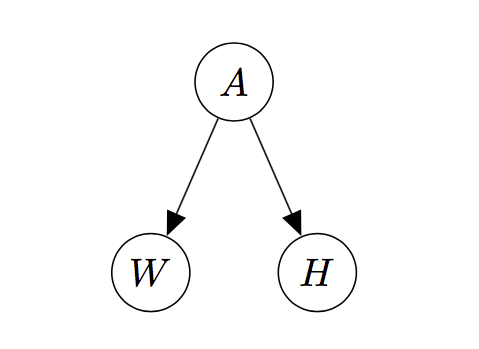
This is sometimes called the “hidden cause graph”, since it indicates that two variables (on the bottom) which are correlated, and which one might be tempted to say have a causal relationship, are in fact caused by some other variable.

Graphical models are useful for keeping track of dependencies in very large distributions. Numerous algorithms for statistical inference, including expectation maximization, belief propagation, certain variational methods, and more, are easily understood in terms of graphical models and algorithms on the underlying graphs.

There is much more to learn with graphical models. For a thorough introduction to this subject, check out this monograph by Martin Wainwright and Michael I. Jordan. However, what we have so far is enough to at least set up channel communcation in graphical form.

Graphical Models of Discrete Channels

For simplicity’s sake, let’s consider a channel that takes in three inputs \(X_1\), \(X_2\), \(X_3\) and spits out three outputs, \(Y_1\), \(Y_2\), \(Y_3\). For now, we make no assumptions about the channel except that it is discrete in time. The graph describing the joint probability distribution of inputs and outputs has lots of edges:

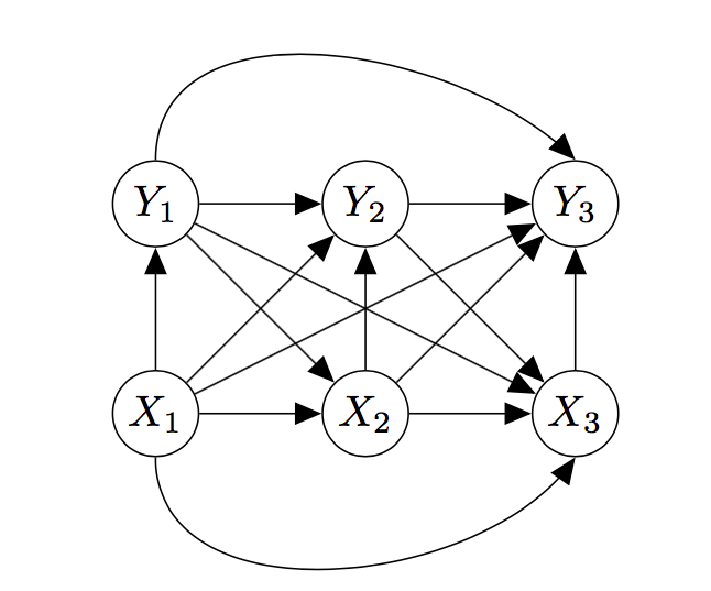
In fact, every node is connected to every other node. This means that none of the variables are conditionally independent of any of the others.

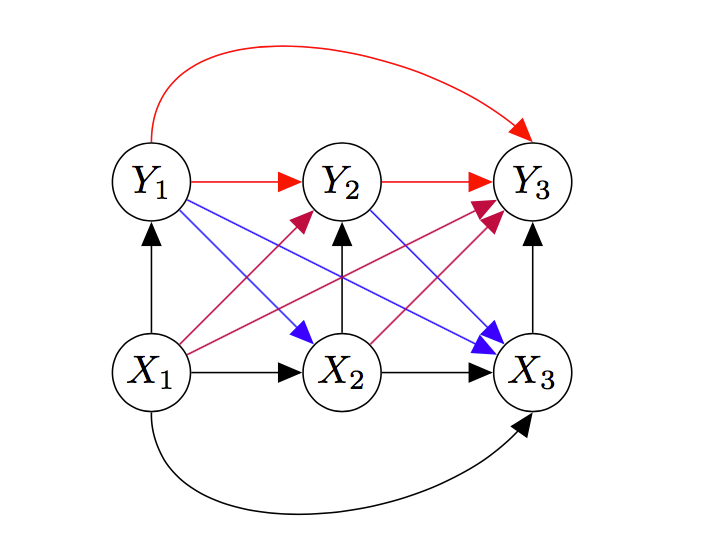
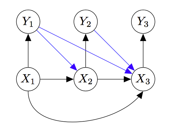
Now, we’ll start making assumptions about the channel. Before doing so, I want to color code the edges, so the following is easier to understand.

First, let’s look at the purple edges (they point from \(X\)s to \(Y\)s). In English, these edges are saying that future values of \(Y\) depend directly on past values of \(X\). That is, even if we know, say, \(X_2\), there is still an effect of \(X_1\) on \(Y_2\). But when we say a channel has no memory, we mean that there is no such effect.

Therefore, for a channel with no memory of past inputs, we can erase those edges, as below.

But the memoryless channel usually has no memory of its past outputs as well – the actual value of its past outputs doesn’t matter for determining future value of the output. \(Y\) values only depend directly on their paired \(X\) value.

Therefore, for a memoryless channel, a channel that has no memory effects on its inputs or outputs, we can erase the red edges, which connect \(Y\) values to each other.

Lastly, channels frequently operate without feedback, which is to say that the actual past values of \(Y\) have no bearing on the future values of \(X\). A television studio doesn’t watch the output on your screen and then adjust the broadcast to compensate for errors.

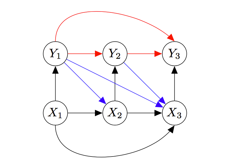
In this case, we can remove the blue edges, which represent direct dependencies of future values of \(X\) on past values of \(Y\).

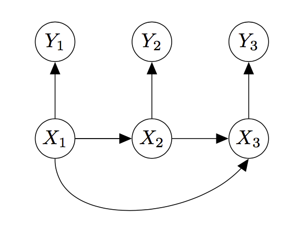
At this point, we can no longer remove any more arrows. In general, the message we are sending has direct dependencies between all symbols, and so the edges connecting the \(X\)s to each other have to stay. Similarly, disconnecting the \(Y\)s from the \(X\)s any further would start to make the \(Y\) sequence independent of the \(X\) sequence, meaning the outputs are independent of the inputs, which is not good for communication.

From this last graph, it is quite easy to read off expressions for the various joint and conditional distributions.

For example, we see that the \(Y\) values are only directly dependent on their current \(X\) values, which means that \(Y_i\) is independent of all other variables, conditioned on \(X_i\)’s value. So the \(Y\) sequence, given the \(X\) sequence, is just a bunch of independent random variables with the same distribution, which we can write as

\[p(y^n\lvert x^n) = \prod_{i=1}^n p(y_i\lvert x_i)\]

Why Graphical Models?

It’s certainly nice to find alternative ways of presenting ideas, especially when that presentation is visual, rigorous, and intuitive. For example, the graphical formulation of linear algebra makes visibly manigest certain abstruse category-theoretic insights into linear algebra. But is there any special utility to thinking about channel communication problems using graphical models?

One big reason is that, as mentioned above, graphical models have been used to explain and develop algorithms for statistical inference in a wide variety of domains, often unifying previously disparate ideas, like the fast Fourier transform algorithm and the belief propagation algorithm. The shared formalism helps us transfer techniques and intuitions from other domains.

If that general idea doesn’t sway you, consider the following: when Shannon first posed the problem of channel communication as above, he was able to quickly and simply prove both that there was a bound on the rate at which information could be communicated and that this rate could be achieved.

What he didn’t do was show a practical way to achieve rates at this limit. In fact, no such method was known for almost 50 years. The method, now known as turbo-coding, was invented by Radford Neal and David MacKay, and the efficient decoding algorithm they proposed was exactly a belief propagation algorithm motivated by viewing the channel coding problem as inference in almost exactly the graphical model presented above, and they described it as such.

Hopefully that convinces you of the utility of the graphical model framework. By making manipulations of probability distributions visual and intuitive, instead of algebraic and rote, it clarifies problems involving probability and inference. In the process, it also unearths deep, surprising connections between different realms of mathematics, enabling the transfer of intuition between domains.