What is information theory? What does entropy measure? Mutual information?
Answer
Information theory provides a set of mathematical ideas and tools for describing uncertainty about the state of a random variable that are complementary to standard methods from probability theory.
Information theory is more useful than standard probability in the cases of telecommunications and model comparison, which just so happen to be major functions of the nervous system!
Among the tools of information theory we find entropy and mutual information. In short, the entropy of a random variable is an average measure of the difficulty in knowing the state of that variable. The mutual information, on the other hand, tells us how much more we know about the state of two random variables when we think about them together instead of considering them separately.
Below, I take a slightly unorthodox approach to the derivation of these quantities, emphasizing the role of modeling and subjectivity in measures of information.
A Problem
In the world of Classical logic as laid out by Aristotle, the comparison of competing claims is simple. If two claims are well-formed, their truth values can be ascertained. A ball is either red, or it is not. When thrown, the ball will either go through the hoop, or it will not. If I claim that when I throw the ball, it will go through the hoop, and you (probably correctly) disagree, I can simply throw the ball to find out who was correct.
There are many claims we wish to make, however, that cannot be admitted to the pristine halls of logical deduction. As David Hume famously noted, inductive reasoning – the sun came up yesterday, and so it shall come up tomorrow – is exactly such a claim, posing serious difficulties for philosophers of science to chew over.
Far from being simply pathological cases, these claims arise quite frequently: for example, despite my poor performance in the past, there was no real reason to believe that it was absolutely, positively false that the ball I threw would go through the hoop – certainly it was not as false as the claim that 2+2=5, or the claim that true is false.
Claims about things that are neither definitely true nor definitely false arise in matters mundane and conseqeuential: producing weather reports, catching the bus, predicting the outcomes of elections, interpreting experimental results, and betting on sports games, to name just a few.
So we would benefit from a method of comparing claims in these situations – which atmospheric model produces better predictions? Is Nate Silver’s FiveThirtyEight a better resource for predicting American presidential elections than the RealClearPolitics aggregator, or talk radio? Are these my lucky dice, or am I just imagining it? Which theoretical model better explains a collection of experimental data points?
Surprise!
The goal, in all the cases above, is to guess about something that we don’t or can’t know directly, like the future, or the fundamental structure of the universe, on the basis of things we do know, like the present and the past, or the results of an experiment.
But we do not seek precise knowledge – in many of these problems, we recognize that exact knowledge, of the kind presupposed and manipulated in Classical logic, is either too difficult or just plain impossible to acquire.
Instead, we seek in these cases to avoid surprise. If I have the correct weather forecast, I am not surprised when it rains at 2 pm – I may have even brought my umbrella. A halo of bent sunlight around Mercury is quite a surprising observation, unless you are Einstein. In contrast, God is never surprised, whereas the unthinkable occurring – 2+2 turning out to be 5, or a particle having negative mass – is infinitely surprising†.
Our mortal inferences, clever or dumb as they are, must have a surprise somewhere between “totally expected”, or 0, and “totally surprising”, or \(\infty\).
We will generally be making statements like: “it will probably rain tomorrow”, or “nine times out of ten, the team with a better defense wins”. This motivates us to express our surprise in terms of probability. If you want a refresher on the foundations of probability, check out this blog post on Bayes’ Rule.
A sort of Occam’s Razor principle will be in effect: if we have two competing models for a phenomenon, like presidential elections, and one is repeatedly declaring the results to be “very surprising” or “probably due to chance”, while the other explains and expects the results, we consider the latter to be more correct. Another related concept from traditional logic would be “special pleading”. The rules of probability, unlike the laws of logic, will allow for the possibility that a freak fluctuation explains the outcomes – that the unlikely occurs – but our method will punish models for relying too heavily on this form of argument.
Put another way, you can imagine that we are playing a prediction game. All players will be given “surprise tokens”, which they allocate out to different outcomes. Any time that outcome occurs, the player takes on that many points – this should remind you of betting*. The goal, as in golf, is to attain the lowest score – a sort of principle of least surprise.
Imagine my friend and I disagree about the shooting performance of the NBA’s long-distance bucket-wizard Steph Curry. Having watched a few Golden State Warriors games, I have come to the conclusion that Curry dominates equally from all positions. My friend disagrees – he thinks that Curry’s shot percentage is lower from the left side of the court than it is in the center or on the right.
If Curry makes a shot from the left, I feel like I’ve won the argument, and if Curry misses, my friend feels the same way. In the world of Aristotle, this causes no trouble: any statement that is part of the world of discourse is either true or false, and we can’t have Curry both making and missing shots from the left. The real world is not so simple: if Curry takes more than one shot, he’s liable to miss some percentage and make some percentage, leaving me and my friend both convinced we are correct.
We resolve this dispute by playing the “surprise game” described above. We each receive a number of surprise tokens. I dole out an equal number to the left, center, and right positions. My friend puts more on the left than in the other two positions, trying to match how much more surprising he finds a successful shot from the left.
We then watch Curry play for several games, taking on surprise tokens every time he makes a shot. After a good number of games have passed, my friend and I compare our tokens. Whoever has fewer tokens – whoever was less surprised – is declared the winner.
This game setup raises a number of questions: what is the optimal strategy for winning the surprise game? How do we allocate our surprise tokens to match our knowledge? Can this be extended to cases where there’s more information available, like the strength of the defense Curry is facing?
Surprise and Probability
Before we can go any further, we need to quantify the relationship between surprise and probability. Our intuition tells us that surprise has some sort of inverse relationship with probability: the victory of a team down by two touchdowns is more surprising than the victory of a team down by a field goal, and it is also less probable.
Furthermore, this increase in surprise happens smoothly as I smoothly decrease probability: if I thought it \(50\%\) likely that my postcard from home would arrive today, it is only marginally less surprising when it does than if I had thought it \(50.00000001\%\) likely (add \(0\)s to taste).
Lastly, we know that an event that is certain to occur has a probability of 1, and when we want to know the probability that any pair events that don’t influence each others’ probabilities occur, we multiply them together. Such events are called “independent events”.
In particular, we can look at the probability that some event \(x\) occurs AND that something that is certain to happen happens. This is just equal to the probability of the original event, \(p(x)\):
where \(C\) is our symbol for an event that is certain to occur – pick your favorite tautology, axiom, or fact.
We can use similar logic to get a rule for surprise. We know that an event that is certain has a surprise of zero. How can we combine \(0\) and some number to get that same number back? We add them!
where I’ve introduced a symbol, \(S\), for surprise.
This combination of rules uniquely defines a function that takes outcomes in and spits out surprises. That function is
Awesome! Check for yourself that all of our criteria above are met: impossible events give infinite surprise, independent events give additive surprises, etc. Note that there is no set base for our logarithm – surprise has no inherent units. If we choose base 2, common in telecommunications, the units are called “bits”, or “binary digits”, whereas the choice of base \(e\), common in statistical physics, gives units called “nats”, or “natural digits”.
You may object to the parasitic definition of surprise here – \(S\) is defined in terms of \(p\), after all. This is an artifact of the historical dominance of the probability approach over the surprise approach. In fact, one can define surprises before probabilities, and define the probability as:
In order to keep the material accessible to as wide an audience as possible, we’ll stick with the parasitic definition. If you’d like to see the major components of the derivation the other way, check out E.T. Jaynes’ Probability Theory: The Logic of Science.
Comparing Surprises
Comparing with Other Models
Let’s return to our original motivation for introducing surprise: comparing competing predictions for events. Every time an event occurs, we can take the probability that each competing model assigns to that event and compute the surprise. One might be tempted to say that the model that was less surprised is the correct one, and move on.
But it is inherent in the kinds of claims we’re considering that one instance isn’t enough – a historic upset in one election isn’t, by itself, cause to throw out all of our intuitions about political science or our data-driven models for election prediction.
But unlikely things shouldn’t usually happen. So if we wish to compare two models, we simply take a look at how surprised they are over repeated instances – repeated experiments, multiple election cycles, several games of basketball. This is precisely the “surprise tokens” game described above.
A lower total surprise is a mark of a better model, and if we want a number that summarizes the surprise we would expect, on average, from a single event, we just divide that total surprise by the number of repetitions:
\[\text{Avg.}\ S_Q = \frac{1}{N} \sum S_q(x)\]where the big \(N\) gives us the number of repetitions, the \(Q\) refers to some particular model, and \(S_q\) refers to the surprise that the model \(Q\) assigns to the event \(x\), derived from its probability distribution \(q\).
In the preceding argument, the notion of repetition played a key role. Unfortunately, repetition is a surprisingly diffcult concept to nail down, much like its partner, probability. If you’re interested in that idea, check out the Aside on Repetition.
Compared with the Truth
Above we took an average over repeated experiments, implicitly assuming that there is a probability distribution over results – that is, after all, the whole motivation for considering probabilistic claims in the first place!
Let’s call that distribution \(p(x)\). This is, in a very real sense, “Nature’s probability distribution”. If that idea sounds strange or unbelievable to you, check out the Aside on Repetition.
With this idea and its new symbol, we can reformulate the relationship above as:
This is the average surprise of the model \(Q\) when its inputs come from the distribution \(p\) of a model \(P\). It is also the limit of the first expression for the average surprise when \(N\) is taken to infinity and so the distribution of the observed events is equal to the true distribution \(p\).
Note that this probability distribution is induced by our experiment and can change – if I know the exact force I apply to a coin to cause it to flip, the result of the toss is no longer 50/50, and so the distribution of results has changed.
This form of the average surprise (you might call it expected surprise, since we’re working with a probability distribution rather than an empirical estimate, so the averaging operation is known as “expectation”), has the advantage of providing exact answers, but the disadvantage of requiring an analytical form for, aka a model of, \(p(x)\), which can be hard to come by.
But if we do have that form, then we can put \(P\) in for \(Q\) in the expression above and get
this is how surprised someone would expect to be, on average, when they have the correct model for the random variable.
It seems intuitively obvious that this average surprise should be the smallest surprise possible – one definition of the correct model might be “the one that is least surprised by the data”. This can, in fact, be shown.
This implies that, for every incorrect model \(Q\), we can figure out how much of its surprise comes from being incorrect and how much comes from the inherent randomness of the process under consideration. We can compute that by just subtracting the average surprise of the correct model from that of our incorrect model, resulting in a measure we might call “excess surprise”:
All of the algebra up there is purely to get the clean-looking final expression – none of it changes the content of the statement, which is that the excess surprise is just the average surprise of the proposed model minus the average surprise of the correct model.
Entropy and Surprise
Now is a good time to take a step back from our exercise here and compare with standard notation and nomenclature.
The average surprise of the model \(Q\) isn’t the usual first step for derivations of information theory. Instead, the average surprise of the correct model is the basic entity. It is known as “entropy” and its symbol, inherited from physics, is \(H\):
Note that the rules of \(\log\) have been used to turn \(\log(1/p)\) into \(-\log(p)\). Why this notation is standard is beyond me, since it emphasizes log-probabilities, rather than the more central notion we call “surprise” and the literature calls “surprisal”, when it deigns to call it anything other than “negative log-probability”.
Since information theory was discovered in the context of telecommunication, and specifically in the context of encoding, decoding, and handling unreliable communication methods, the traditional interpretation of entropy is that it corresponds to the minimum possible average length of an encoded message produced by a source that selects uncoded messages according to the distribution \(P\).
This feels inherently unsatisfying, to me, as a definition for such a basic notion in our understanding of knowledge and inference. But if the communication channel view of entropy and information seems more sensible to you, check out Claude Shannon’s surprisingly accessible original paper deriving the fundamentals of information theory from that perspective.
A reductive but potent view, courtesy of a purely abstract, mathematical approach to probability distributions, interprets the entropy as a measure of the flatness of a distribution: higher entropy means more flat (try out the computation for yourself with a coin that comes up heads and tails with different probabilities). This makes entropy a sort of “summary” of the distribution, just like the mean or the variance.
Contrary to the mathematical and theoretical bent of the above approaches, our choice of basic entity, the average surprise of the model \(Q\), was motivated by an empirical bent – we started with observations \(x\), and models \(Q\) claiming to explain them, rather than with the knowledge of absolute truth implied by \(p\).
This average surprise does have a name in more traditional approaches: it is the cross-entropy of \(Q\) on \(P\). You might see it written:
From the traditional, Shannon perspective, the interpretation of this quantity is that it is the length of encoded messages using a code optimized for a distribution \(Q\) on messages drawn from a distribution \(P\) (can you see why I prefer my approach?). It is used as a cost function to train parametrized models that attempt to predict discrete outputs, also known as classification models.
The final quantity that we derived above, the excess surprise, also appears in both the Shannon approach and in purely mathematical probability. There, it is known as the Kullback-Leibler divergence or the Kullback-Leibler distance. The latter name, though at one point more popular, tends to irritate sticklers for accuracy, since the excess surprise does not satisfy the technical conditions for the mathematical notion of distance. In any case, the most common notation looks something like:
From a mathematical perspective, it is a premetric on probability distributions: it is a primitive notion of distance that captures some basic amount of the structure of the set of probability distributions, and lets us define “convergence in distribution”.
From the Shannon perspective, the KL-divergence is “just the extra bits” when using a sub-optimal coding scheme \(Q\) on messages from \(P\) - a relatively direct connection to our notion of “excess surprise”.
Surprise with multiple variables
Entirely missing from the foregoing has been the discussion of what we can do when we have multiple, possibly related, random variables measured at the same time or during the same experiment– what does the weather in San Francisco tell us about the weather in Berkeley? Vice versa? What about the weather in Beijing? We’d like to say that rain in San Francisco makes rain in Berkeley less surprising, while rain in Beijing does no such thing, but we don’t have the mathematical apparatus for that statement yet.
At the center of this idea is the idea of statistical independence, or the lack of a relationship between two random variables. We’ve encountered this idea already when we defined the additive property of surprise.
Our belief that rain in Berkeley is as (un)surprising with the knowledge that there’s a storm in Beijing as it is without that knowledge is based on just this idea of independence.
If there were a relationship of some kind, we could make a better prediction of, and so be less surprised by, the weather in Berkeley, provided we knew the weather in Beijing and the relationship between the two events.
Since there is a relationship, due to geography, between the weather in Berkeley and the weather in San Francisco, we should expect to be less surprised by the weather in one if we know the weather in the other and the correct relationship between the two events.
This suggests that we should consider an excess surprise, much like the excess surprise between an incorrect model and a correct model, but between the best model knowing both pieces of information and assuming there is no relationship, and the best model with the same information but assuming the correct relationship.
This “correct relationship” is also known as a “joint probability distribution”. Note that, if the “correct relationship” is that the two variables have no relationship, and therefore are independent, the two models are the same and the excess surprise is 0. We also established above that independent probabilities multiply, so the best model assuming independence has a probability distribution that looks like the product of the two individual distributions. In math, that looks like \(p(x,y) = p(x)*p(y)\).
Let’s write this relation out for two variables \(X\) and \(Y\), using \(P_{x,y}\) to refer to the model with the true joint probability distribution and the mathematical symbol \(\bot\) to denote the model that asummes \(X\) and \(Y\) are independent.
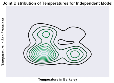
OK, so what does this look like? Let’s imagine that the probability distributions for the weather in Berkeley and San Francisco look like this:
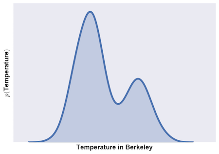
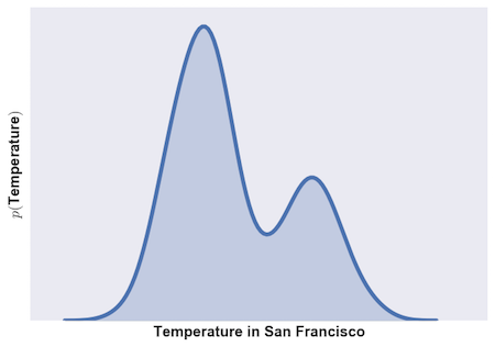
In general, they are temperate cities, but occasionally, things get a bit hot. And what do the joint probabilities look like?
First, how do we visualize joint probabilities? The approach followed below is called a contour plot. The joint probability distribution assigns a value to each point in the \(xy\) plane. Similarly, an elevation map assigns a value, the height, to each point in the \(xy\) plane, where \(x\) is east-west and \(y\) is north-south. Based on this analogy, we steal a tool from cartography: the contour plot. In a contour plot, each colored line traces out a collection of values that have the same elevation, or probability in our case. Darker lines correspond to lower elevations/probabilities.
If we assume that the weather in Berkeley is unrelated to the weather in San Francisco (that is, if we assume independence), then, when we make a contour plot, we get something that looks like the distribution on the left.
If we were to look at this “landscape” from either side, we’d see a bunch of copies of the single-variable distribution, each one scaled to a different height by the probability that the other variable takes that value. This comes from the fact that \(p(x,y) = p(x)*p(y)\): the joint distribution at any value \(y\) is just the distribution \(p(x)\) with its height changed by \(p(y)\).
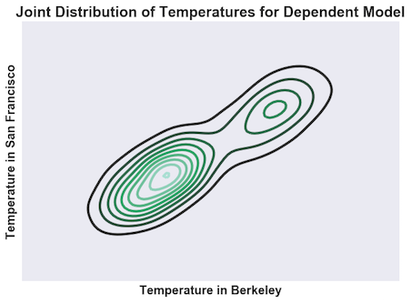
But if we know the true relationship, which is that hot days in Berkeley are also hot days in SF, then we get something that looks like the distribution on the right. Instead of simply having a bunch of scaled versions of \(p(x)\), we have all sorts of different distributions. These are the conditional distributions, \(p(x \lvert y)\), each scaled by \(p(y)\).
This form arises from the equation \(p(x,y) = p(x \lvert y)*p(y)\). The excess surprise measures how big the difference between these two distributions is: a bigger excess surprise means they are more different, and so there is a stronger relationship between the variables. Put another way, the higher the excess surprise, the further the two variables are from being independent.
If you want to know more about conditional distributions, and how Bayes’ Rule is used to manipulate them and model reasoning under uncertainty, check out this blog post.
Surprise and Information
The quantity described above as “the excess surprise from using an independent model of a dependent system”, \(Excess\ S_{\bot}(P_{xy})\), is special enough to get its own name.
It is called the “Mutual Information” between two variables, and it is often denoted \(I(X;Y)\). Because this value expresses how much one variable can tell you about another, it serves as a natural measure of statistical dependence – sort of like correlation, but capable of capturing arbitrarily complex relationships.
It is important to note that, just as correlation does not imply causation, mutual information does not imply causation. The mutual information between the weather and my choice of clothing is the same as the other way around, though only the former causes the latter, so far as I can tell.
Entropy, Information, and Neuroscience
The traditional argument for connecting Information Theory and neuroscience goes something like this: sensory neurons communicate the state of the outside world to the brain, where different layers and brain areas communicate the results of their computations to each other.
As demonstrated by Shannon, there are optimal ways to encode information so that it can be communicated using as little energy as possible and as quickly as possible. These encoding schemes confer an evolutionary advantage on organisms that use them, and so we should expect to find neural codes that are optimal from the perspective of information theory.
The foregoing presentation of the basics of information theory, which emphasizes the role of model-building and model comparison, suggests a deeper connection to neuroscience. The fundamental job of the nervous system is not to merely communicate information efficiently, but rather to construct, from noise-corrupted, ambiguous, and incomplete sensory data, an internal model of the outside world that enables superior action selection for the sake of survival and reproduction.
One should expect, then, that the excess surprise about the state of the outside world of a model that uses observations of neural data, rather than observations of the outside world, should be minimized.
Put another way, if a neuron is representing something about the state of the outside world, the mutual information between that neuron’s state and that part of the world’s state should be high. In fact, one can take that as a sort of definition of what it means for a neuron to “represent” a piece of information about the outside world, like the presence or absence of light at a particular location or the existence of a rewarding stimulus nearby.
There are concerns with this approach: high levels of mutual information are necessary, but not sufficient, for a neuron to represent the outside world. The concerns about causation described above come into play here: a given neuron might be representing a different random variable that happens to be dependent on the same causes as the recorded variable. For example, a neuron that represents conjunctions of contours will have a high degree of mutual information with the individual contours. More concerning still, the neuron might not be engaged in representation at all: even though the state of the glial “helper cells” of the nervous system contains information about the state of the outside world, that information appears as a consequence of the role of glia in regulating gross features (mean activity, etc.) of computation in neurons, where the “representation” truly occurs.
End Matter
In a very real way, no instance is ever repeated: no matter how carefully we control our environment, something will escape our grasp: the barometric pressure, the tone in our voice as we ask a survey question, the arrangement of electrons on Jupiter, or the Hawking radiation emanating from the supermassive black hole at the center of the galaxy.
For all of these confounds, we have no a priori reason to exclude them, and for some, we know they have a (potentially small) effect – Newton’s law of gravitation admits no boundaries.
So instead of getting a precisely repeated instance, we get an instance that is the same so far as we care to know. This leaves nature a little wiggle room for things to be slightly different at the start of our experiment, and so for the results to be different as well.
Famously, the early modern physicist and mathematician Pierre-Simon Laplace stated that, if one only knew the positions, velocities, and masses of all the particles in the world, one could both predict the future state of the universe and know everything about the past. This is untrue, but the picture is helpful.
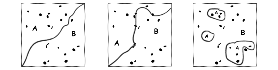
We can imagine, though we cannot hope to write down, the set of all the possible values of the positions, velocities, and masses of all the particles of the universe. An artist’s interpretation of the idea appears below:

We can restrict the set by accepting only those values that are consistent with some fact that we know about some gross state of the world, like “I have a coin perched on my thumb”. In the terms of probability, we call this “conditioning” A sketch of the result of such a conditioning appears below.
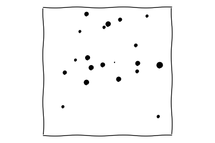
The set of all states of the universe compatible with a statement, e.g. “I have a coin perched on my thumb”.
When I perform my experiment, those values are all definite, but unknown (ignoring, for simplicity’s sake, quantum effects). We assume that, within the subset in which we’ve restrained nature, the distribution of values takes on the flattest distribution that is compatible with our state of knowledge.
This is more than just an act of modesty. It is in fact, a necessity if we are to be intellectually honest. Any less flat distribution would imply that we know more about the possible distributions than we admitted to in our description of our state of knowledge.
As an example of such a distribution: if we know that the values are “around a mean”, in the sense that values further from the mean are always strictly less probable than those close to the mean, the flattest distribution (also known as the “maximum entropy distribution” or the “least informative prior”) is the Normal distribution.
Once we’ve induced a distribution over possible states of the start of an experiment, the laws of nature can take over. These are generally expressed as differential equations, which we usually think of as descriptions of the motion of particles, changing their location, velocity, and mass. They can also move aggregates of particles – that is, they can be applied to our whole list of positions, velocities, and masses – and so they can evolve our initial distribution of states into a final distribution of states.
A possible result of this time evolution appears below. Groups of states have been stretched, shrunk, translated, and rotated by the action of physical laws.
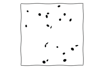
The possible states of the universe after our experiment.
When we, as experimenters, come in and label those states – “heads” or “tails”, “Candidate A won” or “Candidate B won”, “our rocket launched into space” or “our rocket exploded on the launch pad” – we have the distribution over results of our experiment that appears as \(P\) in the main text.
Three possible labelling schemas for the states induced by the experiment above appear in the next figure:
Footnotes
† If this gives you pause, try this out: pick some finite value for how surprising “2+2=5” is. Which is bigger, that value, or the surprise from a coin coming up heads 10 times in a row? 100 times? One billion times? I can do this all day, and I’ll win eventually! The only solution is to make “2+2=5” infinitely surprising.
* In fact, one of the methods for deriving the laws of probability is based on betting. This method, due to de Finetti, is often called the Dutch Book Argument. A “Dutch Book” is a betting strategy that guarantees victory against another player – named after the Dutch due to their reputation as superior financiers, and evincing more than a little Occupy-type sentiment. The correct laws of probability are the only ones against which no Dutch Book exists – a remarkably similar idea to our “surprise tokens” game. A correctly-made model is one that will always win that game against incorrectly-made models.
Acknowledgements
I’d like to thank Jim Crutchfield, especially for his excellent course, Natural Computation and Self-Organization (available online) and Chris Olah, whose blog posts, on information theory and otherwise, were extremely influential.
I’d also like to thank Ryan Zarcone for valuable discussions and for comments on a draft.