What is Bayes' Rule? Explain how an aspect of perception can be expressed in terms of Bayes' Rule.

You can view an updated version of this blog post at this link.

Answer

A note:

I've included a brief primer on probability, with an emphasis on visualization, If you can look at the below image and see \(P(A)\) and \(P(A \& B)\), then the primer isn't strictly necessary, and you can skip to the section "Visualizing Bayes' Rule".

Visualizing Probability

Let's imagine we have two statements about the world, "A" and "B", where sometimes A is true, sometimes B is true, and sometimes A & B are both true. Some examples might be: "It is cloudy" and "It is raining", "I was struck by lightning" and "I was struck by lightning twice", or "I am within 25 miles of Berkeley" and "I am within 25 miles of Stanford".

Now if something isn't definitely true, we say that it is "possibly true" or "probably true". This means that sometimes it happens to be true, and sometimes it does not. If we want to get more specific, we can say that something is "one in a million" or "fifty-fifty", which mean something like "if the same conditions repeated a million times, this statement would be true once/500,000 times"^†.

For any statement, either it or its opposite must be true: it is either raining or it is not, and I was either struck by lightning or I was not. That means that if we set up the same conditions a million times, it will either rain or not rain a million times. This may seem obvious, but it's actually a very important observation!

With that idea in hand, we can move from using numbers to talk about chance to using pictures. Let's draw a square with area 1.

Fig. 1 A square with area 1.

We'll be using this square to represent all the statements that can possibly be true. So an event that always happens, like "It is raining or it is not raining", takes up the whole square, while an event that never happens, like "A is true AND A is false" doesn't take up any space at all. Our intervening cases, like just plain-old "It is raining" or "the coin flip came up heads", take up more space than something that can't be true, but less than something that must be true.

Let's draw the picture for our two generic statements "A" and "B".

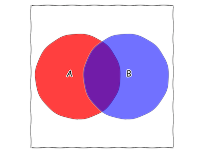
Fig. 2 Two statements that might both be true, represented as areas of our square.

In this case, each circle takes up about 30% of the square. This means that there is a 30% chance that "A" is true. The typical way to write this mathematically is \(\mathbf{P}(A) = \frac{30}{100} = 0.3\) To see the connection between probability and area, you can imagine throwing darts at the square while blindfolded, or throwing grains of sand on the square from above, or counting cosmic ray collisions with the square, and comparing how many are inside the "A" circle with how many are outside the "A" circle.

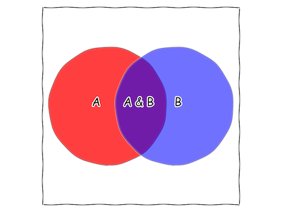
Note that there's a good chunk of the square that is both part of the "A" circle and part of the "B" circle. This new area is called "A&B".

Fig. 3 A new statement appears: "A is true and B is true".

It represents both of our statements being true: "it is cloudy and it is raining", for example, or "this dart landed in the "A" circle and this (same) dart landed in the "B" circle". Is this a good drawing for "I was struck by lightning and/or I was struck by lightning twice"? Why or Why not?

Circles are nice, because we can figure out their area exactly. Unfortunately, not every combination of possibly true statements can be represented by circles: just check out "A&B"!

We can figure out the area by drawing a grid on our square. If our square was like a chessboard, we'd get something like this:

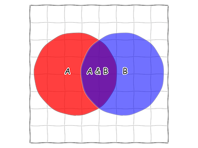
Fig. 4 A chessboard-style 8x8 grid on our square.

We can then note that there are 64 little squares, and 8 of them contain some part of "A&B". Thus, for these statements, it's roughly an 8/64 or 1/8 chance that both "A&B" are true.

But that's just a rough estimate. We can make it better by making the mesh smaller.

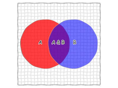
Fig. 5 A 25x25 grid on our square.

And better still by making it smaller still.

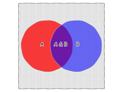
Fig. 6 A 100x100 grid on our square.

You'll notice that there are fewer and fewer squares that have a piece inside "A&B" and so our estimate of the area of "A&B" is based on just counting squares is getting better. If we could make our squares infinitely small, then they'd exactly fill up "A&B" and we could get a perfect estimate of the area of "A&B".

Unfortunately, we don't have time to count infinitely many infinitely small squares, nor is that easy to imagine what they'd look like. The idea should remind you of integrals from calculus, because they're basically the same thing. Just like in calculus, if we can come up with a mathematical formula that represents a statement's area, like "A is a circle with radius 1/2", then we can usually figure out exactly how likely a statement is to be true. Otherwise, we just have to do the equivalent of throwing darts, which statisticians call "sampling".

Visualizing Bayes' Rule

Sometimes, statements will go from being possibly true to being either true or false: when I woke up this morning, there was some chance it was sunny, until I looked out the window and discovered that it was not. From there, I decided it was very probably going to rain, so I grabbed my umbrella on the way out the door. Now, I normally do no such thing, especially when I see that it is sunny.

In this case, it is obvious to everyone why: when there are clouds, there is very often rain. More specifically, it rains more often when there are clouds than when there are no clouds, or when we don't know whether there are clouds.

Bayes' rule is simply a way of formalizing this intution. We can read it right off of a figure like the one below:

Fig. 7 Bayes' rule is hidden in this picture!

To do so, we just need to formalize what it means for a statement to go from possibly true to definitely true. In the previous section, we said that anything that is definitely true has an area equal to the size of our square (let's pick 1, to make our lives easy), while anything that is definitely false has an area 0. Discovering a statement B to be true has the effect of shrinking the area of "B is not true" to 0, while growing the area of "B is true" up to 1.

The result looks something like this:

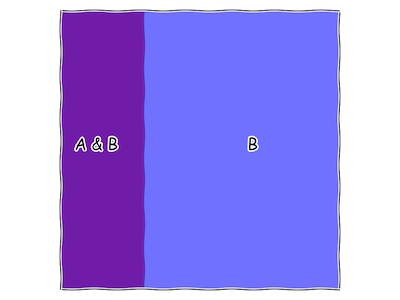
Fig. 8 What our "square of all statements" looks like, once we discover that "B" is true. Note that there is no more red, only purple.

At this point, we can figure out how likely it is that "A" is true, now that we know "B", by measuring its area as a fraction of the square. We call this \(P(A|B)\), which we pronounce "probability that A is true given that B is true". This is also called the "conditional probability of A given B".

We've seen that \(\mathbf{P}(A|B)\) is just the ratio of the size of "A&B" to the size of "B". In mathematical language, this is written:

which we can rewrite as:

Of course, we could've gone the other way around, starting by discovering that "A" was true and then finding the probability that "B" was also true. This would give us a very similar equation to the one above, which we can also rearrange to pull out \(\mathbf{P}(A\& B)\).

We can set out two equations for \(\mathbf{P}(A\& B)\) equal to each other:

And we've now derived Bayes' Rule, which might look more familiar if we rearrange it into:

Bayes' Rule and Learning

At this point, the importance of Bayes' rule, and especially its connection to perception, is yet unclear. Let's pick a few particular kinds of "statement" and put them into Bayes' rule to clear this up. We'll call "B" a "hypothesis" and "A" some "data". Bayes' rule says:

That is, we can figure out how likely a hypothesis about the world is true, given that some data is true. In fact, since we've already seen the data, \(\mathbf{P}(\textrm{Hypothesis | Data})\) is actually our new \(\mathbf{P}(\textrm{Hypothesis})\) – remember that all of the red disappeared, to be replaced by purple, when we conditioned on "B" in Figure 8. We've "updated" our beliefs given some new information. In a very real sense, Bayes' Rule tells you how to learn given the uncertainty and randomness that characterize our apprehension of the world. In fact, there is another path to Bayes' Rule that makes this more explicit (see footnote † for more details).

The probability of our hypothesis is called the "prior probability", and we want to make sure we are as honest and objective in setting this as possible. Concerns that this element was "subjective" in some sense prevented Bayesian methods from catching on in "mainstream" statistics until the late 20th century, despite the fundamental relation being discovered by Bayes in the 18th century and refined by Laplace at the beginning of the 19th. For more on this controversy, see the footnote and references.

The term in the denominator, the probability of the data, caused plenty of trouble as well: finding out the probability of the data means considering every possible hypothesis, which often means doing a nasty, complicated integral. In part because of this, it wasn't until the advent of ubiquitous, powerful computing at the end of the 20th century that the advantages of the Bayesian perspective for problems of scientific modeling were widely recognized and put into practice.

Bayes' Rule and Perception

Finally, we are well equipped to answer the original question: how does Bayes' rule relate to perception? As the preceding section described, it provides a normative account of learning – it describes the optimal way to use incoming data. This is as true for the algorithms Amazon uses to figure out what widgets you're keen to buy as it is for the process by which the brain builds a model of the world by bringing in sensory data.

But Bayes' rule can also be used outside the context of learning. Perception is fundamentally a problem of induction: the data our senses pick up is fundamentally not what we care about. We see a 2-D projection of the oscillations of an electromagnetic field, but want to know the 3-D shape, texture, and color of a rich scene of objects, and we feel minute changes in air pressure inside our skulls, but want to know if they were made by a wolf or a dog.

Here's a concrete example, using our simple picture from above. We're a monkey, living in northeastern India. In the last 100 days, we've heard roaring in the distance 8 times, and been attacked by ferocious White Tigers on 4 occasions. On three of those occasions, we heard roaring in the distance. This morning, we woke up to an ominous rumble. What is the chance that a tiger attacks today?

We can represent this subset of our monkey world with the following diagram:

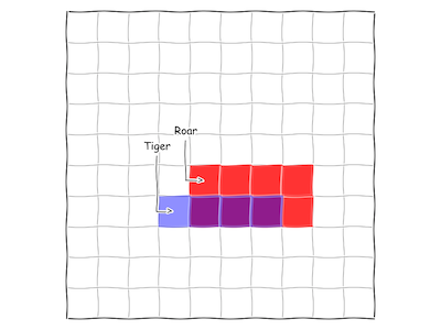
Fig. 9 A small slice of monkey life.

This helps us visualize the three pieces of information we need:

Combining these terms with Bayes' rule:

We now have the information necessary to make an informed decision about whether to ske-daddle or not. This same basic process can be applied to any sensory modality, and to any inductive problem we might ask that modality to solve.

^† A note on frequentism

The section on visualizing probability commits what is a fatal heresy in the eyes of a true, red-blooded Bayesian: it defines the probability of an event in terms of its long-run frequency. This definition is what gave the name to a school of thought that is the perennial nemesis of good Bayesians everywhere: frequentism.

It is certainly possible to avoid this definition. In fact, it is much preferable, since it allows for a normative account that derives Bayesian inference as a natural extension of Aristotelian logic to the case of uncertain premises, with all the power for separating optimal from suboptimal that classical logic provides. Interested readers are pointed to TJ Loredo's From Laplace to Supernova SN 1987A, which Bruno Olshausen described as "practically a religious experience". Extremely interested readers can check out the first few chapters of ET Jaynes' incomplete magnum opus, Probability Theory: The Logic of Science, which gives a full and accessible proof in nearly complete generality.

However, this approach is unwieldy when applied to infinite sets of propositions, especially the uncountable infinities encountered in real-valued spaces, like our humble square. For these, the measure-theoretic approach of Kolmogorov, despite its mathematical austerity and frequentist leanings, is most natural. This is doubly the case in a pedagogical setting, where unwieldy uncountable unions of propositions are likely to confuse students, while the circles and Venn diagrams of the Kolmogorov setting are simply intuitive.

References

On the origins and utility of the Bayesian view of probability:

• Jaynes, ET. Probability Theory: The Logic of Science.

• Loredo, TJ. From Laplace to Supernova SN 1987A: Bayesian Inference in Astrophysics.

On the connection between Bayes' rule and the brain:

• Wolpert D and Gharamani Z, 2006. Bayes rule in perception, action and cognition

• Doya K, Ishii S, Pouget A, and Rao RPN. Bayesian Brain: Probabilistic Approaches to Neural Coding.

• Fiser J, Berkes P, Orbán G, and Lengyel M, 2010. Statistically optimal perception and learning: from behavior to neural representations

Putative psychological and neural evidence of Bayesian perception and action:

• Berkes P, Orbán G, Lengyel M, and Fiser J, 2011. Spontaneous Cortical Activity Reveals Hallmarks of an Optimal Internal Model of the Environment.

• Ernst MO and Banks MS, 2002. Humans integrate visual and haptic information in a statistically optimal fashion.